
Analytical Approaches for Fast Computing of the Thermal Load
of Vehicle Cables of Arbitrary Length for the Application in
Intelligent Fuses
Anika Henke
a
and Stephan Frei
b
On-board Systems Lab, TU Dortmund University, Otto-Hahn-Str. 4, Dortmund, Germany
Keywords: Analytical Approaches, Axial Heat Transfer, Green’s Functions, Intelligent Electronic Fuses, Laplace
Transform, Smart Fuses, Thermal Cable Model, Transient Temperature Computation, Vehicle Cable Systems.
Abstract: In modern intelligent vehicles, a huge number of components leads to complex cable harnesses with high
reliability demands. Static connections protected by simple melting fuses are more and more replaced by
intelligent power distribution and switching units. Thermal considerations play an important role with respect
to reliability as thermal overload situations can lead to accelerated aging, damaged cables and finally to
interruptions in the power supply. The calculation of the axial transient temperature distribution in cable
structures is a complex task that is often solved numerically. In this paper, two analytical approaches to model
the temperature of a single cable in air are presented, that are based on the use of Green’s functions in the
time domain respectively Laplace domain. As sums appear, the convergence behavior is evaluated. The
approaches are validated using a numerical reference solution. The influence of the cable length on the
accuracy of the solutions is examined and complexity considerations are performed. An application example
for intelligent vehicles is presented and discussed.
1 INTRODUCTION
The development of intelligent and connected
vehicles is an ongoing process reaching for improved
safety, efficiency and user comfort. In additional to
established basic functions, a huge variety of features
for automated driving is added. All those features
require highly reliable power supply systems (Kong
et al., 2019) depending on their safety relevance:
Failure in entertainment systems is disturbing but not
critical, whereas failure in safety-critical systems (e.g.
autonomous driving functions) is crucial and must not
appear.
Classically, the electrical power supply is
statically connected to the loads. The connecting
cables are protected with simple melting fuses as
shown in Figure 1(a). During the cable harness
development, those cables and fuses must be
dimensioned considering the maximum expected
currents to avoid overload under all operating states.
Based on an estimated worst-case current pulse, that
a
https://orcid.org/0000-0001-5028-4767
b
https://orcid.org/0000-0002-8917-3914
might appear extremely seldom, an appropriate cable
needs to be chosen. Therefore, cables can be over-
dimensioned for the regular operating states (Horn et
al., 2018). Once under operation, the highly
temperature depending aging process in the cable
begins. Using melting fuses, the duration of a
maximum load condition and the real cable
temperature cannot be monitored, so the remaining
lifetime cannot be estimated.
In recent vehicle developments, intelligent power
distribution units (PDUs) with integrated intelligent
fuses become more widespread (Kong et al., 2019) as
shown in Figure 1(b). Such a PDU can flexibly switch
Figure 1: Power supply in a vehicle using (a) a static
connection with melting fuses or (b) a PDU for flexible and
intelligent switching options.
(a)
(
b
)
396
Henke, A. and Frei, S.
Analytical Approaches for Fast Computing of the Thermal Load of Vehicle Cables of Arbitrary Length for the Application in Intelligent Fuses.
DOI: 10.5220/0010433003960404
In Proceedings of the 7th International Conference on Vehicle Technology and Intelligent Transport Systems (VEHITS 2021), pages 396-404
ISBN: 978-989-758-513-5
Copyright
c
2021 by SCITEPRESS – Science and Technology Publications, Lda. All rights reserved

loads on and off for functional but also fusing
purposes. It is possible to control the power flow
according to safety demands. Thus, highly safety-
critical systems can be prioritized regarding their
power demands. The actual cable insulation
temperature and aging status can be monitored based
on the load history to evaluate the safety of operation
at any time. This enables the operation closer to the
cable limits, i.e. smaller cross sections can be chosen
or temporarily the current can be increased. Therefore,
more options are available in the decision process and
different strategies can be implemented depending on
the safety relevance of the connected systems. For
example, a simple on/off switching strategy can be
used that interrupts the current if a predefined
temperature limit is exceeded and switches it on again
as soon as the temperature falls below a second
defined temperature as e.g. mentioned in (Önal et al.,
2020). So, the usage of an intelligent fuse can enhance
the availability and reliability of the complete system
or reduce its weight as over-dimensioned cables can
be avoided. To enable a reasonable switching
decision, the cable insulation temperature has to be
known.
As the insulation temperature often cannot be
measured directly, thermal cable models based on
current measurements are necessary. If additional
information (e.g. the environmental temperature) is
available, it can also be considered. Otherwise, worst-
case assumptions are necessary.
Thermal cable models to be integrated into PDUs
with cheap and less powerful microcontrollers should
be as simple as possible. Very basic analytical models
that neglect the axial heat flow along the cable (e.g.
(Zhan et al., 2019) or (Olsen et al., 2013)) or the
transient temperature development (e.g. (Brabetz et
al., 2011) or (Holyk et al., 2014)) cannot predict the
cable temperature very precisely. More complex
models are often based on a two- or three-
dimensional model of the cable which is used for the
numerically based simulation of the cable
temperatures as, e.g., in (He et al., 2013). Nearly
arbitrary environmental and load conditions can be
modelled this way, but these methods require high
computational effort. This effort can be drastically
reduced by using analytical methods. In this paper,
two different methods for analytical temperature
calculations using Green’s functions are presented
and discussed. Those allow a precise temperature
calculation with low effort for a single insulated cable
under special conditions based on the known current.
In chapter 2, the fundamental model is presented.
Earlier research is shortly summarized. The new
analytical solution methods based on the use of
Green’s functions in the time domain respectively
Laplace domain are introduced in chapter 3. In
chapter 4, those new methods are validated and
compared to earlier developed methods with regard to
their performance. In chapter 5, an application
example is discussed: Failure leads to an overcurrent
that causes a melting fuse to trip. Unlike, with an
intelligent fusing strategy, the overload can be
tolerated, and important automated driving
applications can still be provided. An uncontrolled
system breakdown is avoided.
2 PRELIMINARY WORK
This section is based on (Henke and Frei, 2020).
There, the fundamental model was presented for a
single cable of length 𝐿 oriented in 𝑧-direction con-
sisting of a conductor (radius 𝑟
) and an insulation
(outer radius 𝑟
) as shown in Figure 2(a). A current 𝐼
flows through the cable. The equivalent circuit for an
infinitesimally short cable segment shown in Figure
2(b) is used. Per unit length (pul) quantities are
marked with an upstroke. The pul heat source 𝑃
represents the cable heating induced by the current 𝐼
that flows through the conductor and depends on the
conductor temperature 𝑇. The pul capacitance 𝐶
is
used to model the heat storing capacity of the
complete cable (conductor and insulation). The pul
admittance 𝐺
describes the heat conduction through
the insulation layer and the heat transfer from the
cable to the ambient air via convection and radiation
and depends on the cable surface temperature 𝑇
and
the ambient air temperature 𝑇
. The axial heat flow in
the conductor is modelled using the pul resistance 𝑅
.
The axial heat flow in the insulation is neglected due
to the low thermal conductivity of the insulation
compared to the conductor.
Figure 2: (a) Examined single cable. (b) Thermoelectric
equivalent circuit for infinitesimally short cable segment.
From this equivalent circuit, the partial differential
equation (1) is derived for the conductor temperature
𝑇
𝑧,𝑡
with the initial and boundary conditions (2).
𝜕
𝑇𝜕𝑧
⁄
−
𝐴
𝜕𝑇 𝜕𝑡
⁄
−𝐵𝑇=−𝐶,
(1
)
𝐴
=𝑅
𝐶
,𝐵 =𝑅
𝐺
,𝐶 = 𝑅
𝐺
𝑇
−𝑃
,
𝑇
𝑧,0
=𝑇
,𝑇
0,𝑡
=𝑇
,𝑇
𝐿,𝑡
=𝑇
.
(2
)
(a) (b)
Analytical Approaches for Fast Computing of the Thermal Load of Vehicle Cables of Arbitrary Length for the Application in Intelligent
Fuses
397

This differential equation can be solved using the
Laplace transform. In the Laplace domain, an
ordinary differential equation remains, and an
analytical solution is found. Using the approximation
(3), which is valid for long cables (large 𝐿), the
analytical expression (4) in the time domain is
calculated.
𝑒
± 1≈±1,
(3)
𝐷
𝑧
=er
f
𝑧
𝐴
4𝑡
⁄
(4)
𝐷
𝑧
= 𝑒
|
|
√
er
f
𝐴
|
𝑧
|
−2
√
𝐵𝑡
2
√
𝐴
𝑡
−1
+𝑒
|
|
√
erf
𝐴
|
𝑧
|
+2
√
𝐵
𝑡
2
√
𝐴𝑡
−1,𝑧
=𝐿−𝑧,
𝑇
𝑧,𝑡
=
𝐶
𝐵
+
𝐶
𝐵
−𝑇
𝑒
1−𝐷
𝑧
−𝐷
𝑧
+
𝐶
𝐵
−𝑇
𝐷
𝑧
2
+
𝐶
𝐵
−𝑇
𝐷
𝑧
2
.
As already mentioned above, the parameters 𝑃
and 𝐺
in the equivalent circuit are not constant but
depend on the cable and surface temperatures. This
nonlinear dependency was neglected in the above
presented solution. To take it into account, an
iterative solution approach was developed in (Henke
and Frei, 2020) and is shortly resumed here: After an
initialization, the surface temperature 𝑇
and the
parameters 𝑃
and 𝐺
are calculated. Those are used
to find the conductor temperature 𝑇. As termination
condition, the absolute difference 𝜎
=
|
𝑇
−𝑇
|
between two iterations is calculated. The process is
continued until this difference falls below Δ
,
=
0.001 K. In Figure 3, this approach is summed up.
Figure 3: Iterative approach for nonlinearities.
3 APPROACHES BASED ON
GREEN’S FUNTIONS
In this section, two new approaches for the solution
of the partial differential equation (1) are presented.
Both of them are based on Green’s functions.
3.1 Time Domain Approach
In this approach, Green’s functions are used to solve
the partial differential equation directly in the time
domain. The problem can be classified as
inhomogenous differential equation with
inhomogenous boundary and initial conditions as
generally, 𝐶, 𝑇
, 𝑇
and 𝑇
are not zero. According to
the principle of superposition, the complete solution
results as superposition of solutions that take into
account only one of the inhomogeneities assuming
the others to vanish:
𝑇
𝑧,𝑡
=𝑇
|
+𝑇
|
+𝑇
|
+𝑇
|
(5)
From the corresponding Green’s function (6), the
different solution parts (eq. (7)) are calculated. The
solution for 𝑇
≠0 is calculated using the solution
for 𝑇
≠0 by replacing 𝑇
with 𝑇
and 𝑧 with 𝐿−𝑧
due to symmetry considerations. The superposition of
all four parts leads to the complete solution (8).
𝐿
=2𝑛𝐿,𝐺
𝑧,𝑡
|
𝑧
,𝜏
=
𝑒
√
−
𝐴
2
𝜋
𝑡−𝜏
⋅
𝑒
−𝑒
,
(6)
𝑇
|
=𝐺
𝑧,𝑡
|
𝑧
,0
𝑇
d𝑧
,
(7)
𝑇
|
=𝐺
𝑧,𝑠
|
𝑧
,0
𝐶 d𝑧
d𝑠
,
Ψ
𝑧,𝑡
=
−1
𝐴
𝜋𝑡
⁄
𝜕
𝑒
,
𝑇
|
=Ψ
𝑧,𝑠
𝑇
d𝑠
.
𝑇
𝑧,𝑡
=𝑇
𝑧,𝑡
(8)
+
𝐶𝐵
⁄
−𝑇
𝑒
⁄
𝐷
−𝑧
+𝐿
+𝐷
−𝑧
−𝐿
−𝐷
𝑧+𝐿
−𝐷
𝑧−𝐿
+0.5
𝐶𝐵
⁄
−𝑇
𝐷
𝑧+𝐿
− 𝐷
𝑧−𝐿
+
𝐶𝐵
⁄
−𝑇
𝐷
𝑧
+𝐿
−𝐷
𝑧
−𝐿
.
Here, the earlier term from the solution in the Laplace
domain 𝑇
𝑧,𝑡
appears again and is extended by
additional terms. This new solution is complete, as no
approximations were necessary. Nevertheless,
because of the infinite sum, in an implementation
only a finite number of terms can be considered,
which results in an approximation.
3.2 Laplace Domain Approach
The second new approach operates in the Laplace
domain as the earlier described solution. There, some
terms caused problems with the transform back into
the time domain as expressions with several
exponential functions depending on
√
𝑠
needed to be
true
false
end
initialization
VEHITS 2021 - 7th International Conference on Vehicle Technology and Intelligent Transport Systems
398

transformed. To avoid this problem, using Green’s
functions, expressions are derived, that can be
transformed back into the time domain more easily.
This approach is used in the electrical transmission
line theory as well (Antonini, 2008). For homogenous
boundary conditions (9) the conductor temperature
𝑇
is calculated via eq. (10) from the Laplace
domain Green’s function 𝐺
of the problem (11).
0=𝑇
𝑧,𝑠
|
=𝑇
𝑧,𝑠
|
,
(9
)
𝑇
𝑧,𝑠
= −𝐺
𝑧,𝑧
,𝑠
𝐼
d𝑧
,
𝐼
=
𝐴
𝑇
+𝐶 𝑠
⁄
.
(10)
𝐺
𝑧,𝑧
,𝑠
=−
2
𝐿
𝜓
𝑧
𝜓
𝑧
𝑠𝐴 + 𝐵
+𝑛
,
𝜓
𝑧
=sin
𝑛
𝑧
,𝑛
=𝑛𝜋𝐿
⁄
.
(11)
A series approach for the Green’s function is used
instead of the direct usage of the Green’s function of
the Helmholtz equation. This way, the result in the
Laplace domain (12) can easily be transformed back
into the time domain (see eq. (13)).
𝑇
𝑧,𝑠
=
4𝐼
𝐿
sin
𝑚
𝑧
𝑠𝐴 + 𝐵
+𝑚
1
𝑚
,
𝑚
=
2𝑚+ 1
𝜋𝐿
⁄
.
(12)
𝑇
𝑧,𝑡
=4𝐿
⁄
⋅ sin
𝑚
𝑧
𝑚
⁄
(13)
⋅𝑇
𝑒
+𝐶
1−𝑒
𝐵+𝑚
.
By now, homogenous boundary conditions were
assumed. The result can be applied for inhomogenous
boundary conditions (14) by setting the reference
temperature to 𝑇
=𝑇
. If the cable end temperatures
are not equal, the expansion (15) is necessary. The
transformation back into the time domain leads to eq.
(16). The boundary conditions at 𝑧=0 m and 𝑧=𝐿
are fulfilled for the limit (17), but this solution is
unsteady at the cable ends.
𝑇
𝑧,𝑡
|
=𝑇
=𝑇
𝑧,𝑡
|
=𝑇
≠0
(14)
𝑇
,
𝑧,𝑠
=
𝑇
𝑠
d
d𝑧
𝐺
𝑧,𝑧
,𝑠
|
(15)
−𝑇
𝑠
⁄
dd𝑧
⁄
𝐺
𝑧,𝑧
,𝑠
|
+𝑇
𝑧,𝑠
𝑇
,
𝑧,𝑡
=𝑇
𝑧,𝑡
(16)
+
2
𝜋
1−𝑒
𝑛
sin
𝑛
𝑧
𝑛
𝑛
−𝐵
𝑇
−
−1
𝑇
lim
→
𝑇
,
𝑧,𝑡
=𝑇
,lim
→
𝑇
,
𝑧,𝑡
=𝑇
.
(17)
Additionally, the expansion converges slowly (see
section 4.3). So, the practical applicability is limited.
4 VALIDATION
In this section, the derived approaches are evaluated.
If not stated differently, the following 6 mm
-cable
is evaluated: The solid copper conductor has the
radius 𝑟
=1.382 mm, the specific heat capacity
𝑐
=3.4⋅10
J/m
K, the thermal conductivity 𝜆
=
386 W/Km and the resistivity 𝜌=1.86⋅ 10
Ωm
at 20 °C. The linear temperature coefficient is 𝛼
=
3.93 ⋅ 10
1/K. The conductor is surrounded by a
PVC insulation. The total radius of the cable with
insulation is 𝑟
=2 mm. The specific heat capacity of
the insulation material is 𝑐
=2.245⋅ 10
J/m
K, the
thermal conductivity is 𝜆
=0.21 W/Km and the
emissivity is 𝜀=0.95. The examined cable is loaded
with the current 70 A. 25 °C is the environmental
temperature 𝑇
, which is as well the temperature of
the whole cable at 𝑡=0 s (𝑇
). The beginning (𝑇
)
and the end (𝑇
) of the cable have the temperature
50 °C.
As reference solution 𝑇
, the numerical
solution of the partial differential equation (1) of the
problem is calculated using the function pdepe of
MATLAB (MathWorks, 2020). Generally, partial
differential equations of the form (18) with initial
conditions 𝑢
𝑥,0
and boundary conditions (19) are
solved by this function. As in the concrete problem,
the cable surface temperature 𝑇
is necessary for the
calculation of the parameters of the equivalent circuit,
the formulation (20) is implemented. The nonlinear
material parameters are directly considered here, so
further iterations are not necessary.
𝑐
𝑥,𝑡,𝑢,𝜕𝑢 𝜕𝑥
⁄
𝜕𝑢 𝜕𝑡
⁄
=𝑠
𝑥,𝑡,𝑢,𝜕𝑢 𝜕𝑥
⁄
+𝑥
𝜕
𝑥
𝑓
𝑥,𝑡,𝑢,𝜕𝑢 𝜕𝑥
⁄
𝜕𝑥
⁄
(18
)
𝑝
𝑥,𝑡,𝑢
+𝑞
𝑥,𝑡
𝑓
𝑥,𝑡,𝑢,𝜕𝑢 𝜕𝑥
⁄
=0
(19
)
𝑢=
𝑇𝑇
,𝑥=𝑧,
(20
)
𝐴
𝜕𝑇 𝜕𝑡
⁄
=𝜕
𝑇𝜕𝑧
⁄
−𝐵
𝑇
𝑇+𝐶
𝑇,𝑇
,
0=0+𝑇−𝑇
−𝑅
𝑇−𝑇
𝐺
𝑇
.
4.1 Convergence Behavior
In Figure 4, the convergence of the sums appearing in
the above presented solutions is evaluated. The
deviation from the numerically calculated temperature
Δ𝑇=𝑇− 𝑇
is shown here. A cable of the very
short length 𝐿=0.1 m is examined as later on in this
paper, it is shown, that especially for short cables, the
new solutions drastically improve the accuracy of the
predicted temperatures. For comparison, the results
calculated via the old approximation solution are
given. As can be seen, those lead to much higher
deviations than the new solutions. The series solution
derived via Green’s functions in the time domain and
the series solution for 𝑇
=𝑇
from the Laplace
Analytical Approaches for Fast Computing of the Thermal Load of Vehicle Cables of Arbitrary Length for the Application in Intelligent
Fuses
399
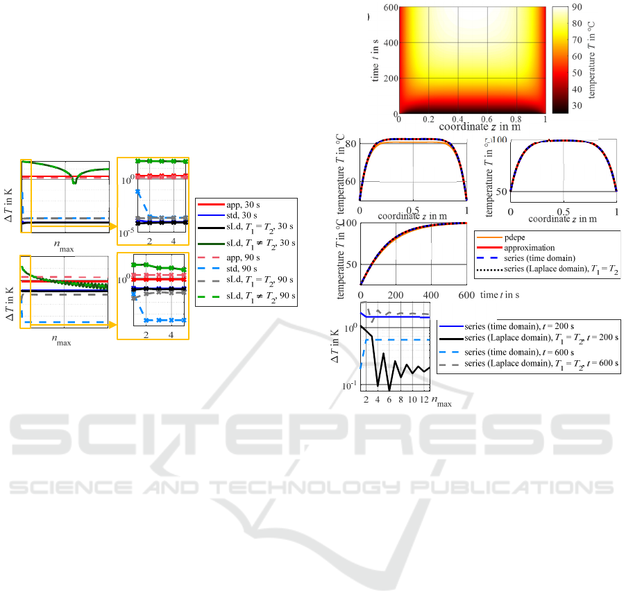
domain converge very fast. Unlike, the series solution
considering the boundary conditions 𝑇
≠𝑇
shows a
bad convergence behavior. In this solution, instead of
the position 𝑧=0 m, the slightly higher value 𝑧=
1 mm is inserted in the calculation because of the
unsteady behavior of the solution at this position.
Because of the bad convergence, this solution is not
applicable for the solution of real problems and will
not be further evaluated in the following.
Figure 4: Deviation between analytically (approximation
(app), series time domain (std), series Laplace domain
(sLd)) and numerically calculated temperatures depending
on the number of addends at (a) the beginning and (b) the
middle of the cable.
4.2 Validation with Numerical Solution
Now, a cable with the length 𝐿=1 m is evaluated. In
Figure 5(a), the cable temperature calculated with the
numerical reference solution is shown depending on
the time 𝑡 and the spatial coordinate 𝑧. In Figure 5(b),
for three cases, the results calculated via the
numerical reference solution and via the three
analytical solutions are compared: The transient
temperature development is evaluated at 𝑧=0.5 m
(middle of the cable). For the times 𝑡=200 s
(transient area) and 𝑡=600 s (stationary), the axial
temperature development along the cable is evaluated.
Here, for the new solution “series (time domain)”
based on the Green’s functions in the time domain,
only one addend from the sum is taken into account,
for the solution based on the Green’s functions in the
Laplace domain (“series (Laplace domain)”), 10
addends are used. As shown in Figure 5(c) for the
position 𝑧=0.5 m, convergence is not reached for
this number of terms. Nevertheless, the usage of so
few terms is evaluated here as in practical
applications, also only a low number of terms can be
considered due to restricted calculation power. All of
the presented solutions show a similar development.
So, for this case, all three solutions can be used.
Figure 5: Results for the cable length 1 m. (a) Numerical
reference solution. (b) Results for fixed position
respectively time. (c) Convergence behavior example.
For a very short cable, the approximation used in
the solution from the Laplace domain (Henke and Frei,
2020) is not valid anymore. That is why for short
cables, huge deviations between the old solution and
the reference solution are expected. To evaluate
theperformance of the newly derived solutions, the
calculation is repeated for a cable with the length 𝐿=
0.1 m. In Figure 6, the results are presented. Because
of the short cable length, the conductor temperature in
the middle of the cable is much lower than before as
the cable ends cool the cable in this example (see
Figure 6(a)). In Figure 6(b), it is shown, that the
solution resulting from the Laplace domain without
Green’s functions is not able to model the temperature
development correctly, but, as expected, massive
deviations appear. The set boundary conditions at the
cable ends are not fulfilled anymore. If just one
addend of the sum resulting from the Green’s function
solution in the time domain (solution “series (time
domain)”) is added, the result matches to the
numerical reference solution much better. The
solution based on Green’s functions in the Laplace
domain (“series (Laplace domain)”) also predicts the
correct temperatures quite well. As can be seen for the
05
0
10
0
1
0
-5
10
0
05
0
10
0
1
0
0
(b)
(a)
(a)
(c)
(b)
𝑡=200 s
𝑡=600 s
𝑧=0.5m
𝑧=0.5m
VEHITS 2021 - 7th International Conference on Vehicle Technology and Intelligent Transport Systems
400
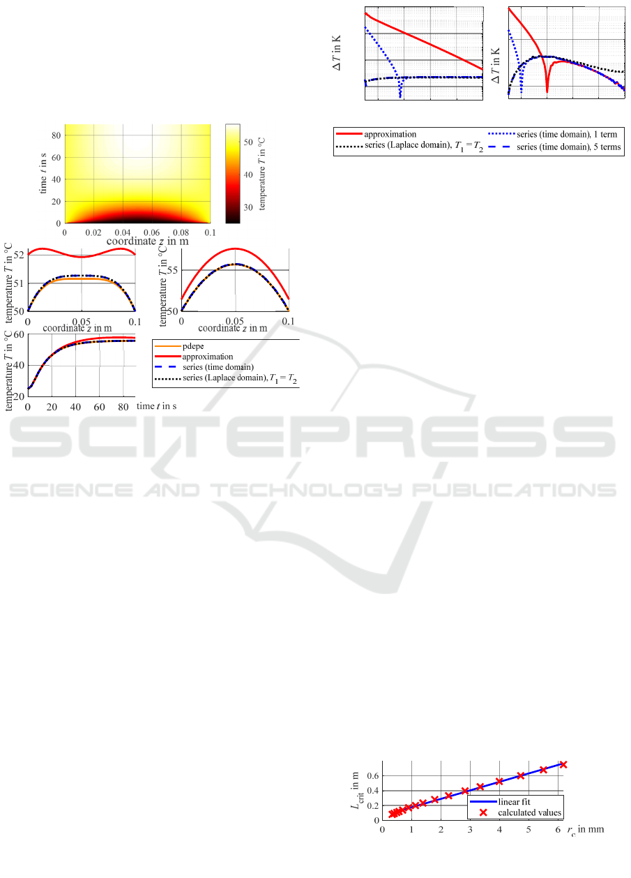
time 𝑡 =30 s, in the transient case, both series
solutions show noticeable deviations to the numerical
reference solution, but those are much lower than 1 K.
Furthermore, the set boundary con-ditions are fulfilled
by both solutions. So, all in all, for this very short cable,
the usage of the new series solutions massively
improves the accuracy of the predicted temperatures.
Figure 6: Results for the cable length 0.1 m. (a) Numerical
reference solution. (b) Results for fixed position
respectively time.
4.3 Influence of the Cable Length
As shown in Figure 6, for short cables, the
approximation causes deviations from the numerical
solution. For the stationary case, even the set boundary
conditions (cable end temperatures) are not calculated
correctly. In Figure 7, this effect is studied. The
dependency of the deviation between the different
analytical solutions and the numerical reference
solution from the cable length is presented for the time
𝑡=1000 s at the beginning of the cable (𝑧=0 m)
and in the middle of the cable (𝑧=0.5 𝐿). As can be
seen for the cable beginning, for short cables, the
deviation of the Laplace approximation grows
exponentially. Using the new solutions based on the
usage of Green’s functions in the time domain by
simply adding one more term improves the results, but
for cable lengths below 0.4 m, rising deviations
appear as well. Using more terms (shown for 5
addends here) ensures a stable behavior in the
complete evaluated area down to 0.1 m. The same
behaviour is also observed using the series solution
from the Laplace domain for identical cable end
temperatures 𝑇
=𝑇
(10 addends). In the middle of
Figure 7: Deviation between the analytically and
numerically calculated temperatures depending on the cable
length at (a) the beginning and (b) the middle of the cable.
the cable, also, for short cables, using the new
solutions improves the accuracy of the solution. For
longer cables, the series solution from the Laplace
domain shows a worse accuracy. Here, more terms
need to be taken into account to improve this. So
especially for short cables, the new solutions can
improve the results. By changing the number of
addends that is used in the solutions, the accuracy of
the solutions can directly be adapted.
Also, the cable cross-section area influences the
deviations. A critical cable length 𝐿
is introduced,
under which the Laplace approximation cannot be
used any longer. This critical cable length is defined
as the cable length, at which the deviation for the
stationary temperature in the middle of the cable
exceeds 3 K. The critical cable length is calculated for
different cables that are characterized by their
conductor radius 𝑟
. For each cable length, the current
through the cable is chosen so that the stationary
temperature in the middle of the cable is
100 ±
0.2
°C. Using the bisection method, this current and
the corresponding critical cable lengths are found. For
the cable length, an uncertainty of 1 mm is allowed as
stop criterion. The results are shown in Figure 8. A
linear correspondence between the critical cable
length and the conductor radius is observed: The
smaller the cable conductor radius, the shorter the
critical cable length is. So especially for short cables
with a high cross section, the approximation from
(Henke and Frei, 2020) cannot be used as its accuracy
is very bad there. Then, the new solutions can replace
this method as analytical calculation approaches.
Figure 8: Critical cable length depending on conductor
radius.
(a)
(b)
𝑡=30 s
𝑡=90s
𝑧=0.05 m
0.2 0.4 0.6 0.8 1
L in
m
10
-4
10
-2
10
0
10
2
0.2 0.4 0.6 0.8 1
L in
m
10
-2
10
0
(a) (b)
Analytical Approaches for Fast Computing of the Thermal Load of Vehicle Cables of Arbitrary Length for the Application in Intelligent
Fuses
401

4.4 Complexity Considerations
The numerical complexity has a major impact on the
runtime and practical applicability. Here, for the
analysis of the complexity of the different solutions,
only the appearance of functions as the exponential
function, the error function or the sine in the final
calculation formula are compared. The square root
and the calculation of the cable parameters are not
considered here. In the solution from the time
domain, the approximation from the Laplace domain
without Green’s functions (11 function evaluations)
appears again. Each additional term from the sum
goes with 20 function evaluations. Compared to that,
the evaluation of a single term from the solution from
the Laplace domain Green’s functions takes much
less effort (2 function evaluations). This rough
estimation of the complexities of the different
approaches also motivates the above used number of
terms: Taking one additional term into account for the
series solution in the time domain results in a total
number of 31 function evaluations, whereas 20
evaluations are necessary for the series solution in the
Laplace domain. So, although a higher number of
addends is taken into account, the series solution in
the Laplace domain causes less calculation effort.
5 APPLICATION EXAMPLE
The standard ISO 6722 defines critical insulation
temperatures based on the insulation aging due to
thermal stress. For PVC, the continuous operation
temperature (3000 hours) is 𝑇
=105 °C. The
corresponding short-term temperature (240 hours) is
𝑇
=130 °C and the thermal overload
temperature (6 hours) is 𝑇
=155 °C. So, on the one
hand, higher temperatures drastically reduce the
expected lifetime of the insulation material. On the
other hand, this means that thermal overload can be
tolerated for a short time, if necessary, but the
accelerated aging has to be considered. In Figure 9,
the insulation lifespan is presented depending on the
insulation temperature. For temperatures higher than
𝑇
, a degradation of the insulation occurs even after
short times. If the temperature becomes higher than
𝑇
, the insulation can start to burn and operation is
not possible at all. Melting fuses are supposed to keep
the cable temperature in the dark green area, short-
time overload situations that lead to accelerated cable
aging (light green area) or the need to replace the
cable afterwards (yellow area) cannot be tolerated.
Unlike, intelligent fuses can support controlled
overload situations.
In Figure 10, a possible use-case for overload
handling using simple melting fuses on the one hand
and intelligent fuses on the other hand is presented. In
case of a simple melting fuse, if the fuse trips, a hard
interruption of functions results, which causes an
undefined and potentially unsecure state of the
complete system. Using an intelligent fuse, the
overload is detected but the cable is not directly
disconnected. First, the advanced driver assistance
systems (ADAS) controller is asked whether an
emergency operation is necessary. In case of a
requested emergency operation the cable can be
operated in the light green or even yellow area of
Figure 9. This way, in many cases, a defined and safe
state can be achieved by controlled measures, and
afterwards it can be decided whether the cable has to
be replaced. The safety and reliability of the complete
system is massively improved.
Figure 9: Lifespan of the cable insulation depending on the
insulation temperature with different operating regions.
Figure 10: Overload handling with (a) melting fuses and
(b) PDUs in combination with intelligent fuses.
An example is shown in Figure 11: A 48 V ADAS
controller has a power consumption of 2 kW. The
power supply is realized via a PDU with intelligent
fuses. The cable that connects the PDU and the
ADAS controller has a length of 3 m and is
dimensioned for a rated current of 42 A. Maximum
environmental and contact temperatures of 𝑇
=𝑇
=
𝑇
=85 °C are assumed. Then, to ensure a
temperature below 𝑇
=105 °C, a cable with a
cross-section area of 10 mm
is necessary (stationary
maximal cable temperature: 99.0 °C). It is assumed
now that due to a failure the power consumption of
(a)
(b)
VEHITS 2021 - 7th International Conference on Vehicle Technology and Intelligent Transport Systems
402

the ADAS controller rises to 4 kW at 𝑡=0 s, but
essential functions still work (partial failure). Then,
the current through the cable rises as well: 𝐼
≈
83 A. Assuming an initial cable temperature of
100 °C, the corresponding cable temperature deve-
lopment in the middle of the cable (hottest spot) is
shown in Figure 12. After 27 s , the temperature
𝑇
=105 °C is reached. A melting fuse would
break the circuit here to protect the cable and
automated driving applications would not be possible
any longer. In contrast, in an intelligent fusing PDU,
the actual cable temperature and cable aging can be
considered: The short-term temperature 𝑇
=
130 °C is reached after about 290 s. The critical ther-
mal overload temperature 𝑇
=155 °C is not
reached at all as the maximum longterm temperature
is 138 °C. Therefore, an intelligent fuse does not trip,
but monitors the cable aging. Automated driving is
still possible, and the vehicle can be transferred into a
safe state by performing a controlled shutdown.
Figure 11: Simple application example for the use in
intelligent vehicles.
Figure 12: Cable temperature development for the
application example.
6 CONCLUSIONS
In this paper, two new approaches for the analytical
transient axial temperature calculation of single
cables were presented. Those approaches are based
on the use of Green’s functions in the time domain
respectively Laplace domain. The results are series
representations. By choosing an appropriate number
of addends, a high accuracy of the proposed methods
can be obtained even for short cables. A constant
cable temperature at the beginning of the calculation
time, constant cable termination temperatures, a
constant current through the cable and a constant
ambient temperature are assumed. Regarding
applications for example for intelligent vehicles, the
presented solutions can be used as fast approach for
the temperature calculation in cables and therefore
provide a basis for decisions in time- and safety-
critical environments.
The presented example shows the potential of
analytical solutions that can deal with limited
resources and still model the essential thermal effects
with an accuracy that allows them to be used in
protective applications. In the example, a melting fuse
would break the circuit due to an overcurrent and
automated driving would not be possible any longer.
Unlike, using a smart fuse with the presented
analytical methods, the overcurrent can be tolerated
and a controlled shutdown is enabled.
ACKNOWLEDGEMENTS
The work for this contribution was partly financed by
the European Fund for regional development (EFRE),
Ministerium für Wirtschaft, Innovation, Digitali-
sierung und Energie of the State of North Rhine-
Westphalia as part of the AFFiAncE project.
REFERENCES
Antonini, G., 2008. A Dyadic Green’s Function Based
Method for the Transient Analysis of Lossy and
Dispersive Multiconductor Transmission Lines. In
IEEE Trans. Microw. Theory Techn., 56(4), 880-895.
Brabetz, L., Ayeb, M., Neumeier, H., 2011. A new
approach to the thermal analysis of electrical
distribution systems. In SAE Technical Paper.
He, J., Tang, Y., Wei, B., Li, J., Ren, L., Shi, J., Wu, K., Li,
X., Xu, Y., Wang, S., 2013. Thermal Analysis of HTS
Power Cable Using 3-D FEM Model. In IEEE Trans.
Appl. Supercond., 23(3), 5402404-5402404.
Henke, A., Frei, S., 2020. Transient Temperature
Calculation in a Single Cable Using an Analytic
Approach. In JFFHMT, 2020(7), 58-65.
Holyk, C., Liess, H.-D., Grondel, S., Kanbach, H., Loos, F.,
2014. Simulation and measurement of the steady-state
temperature in multi-core cables. In Electric Power
Systems Research, 116, 54–66.
Horn, M., Brabetz, L., Ayeb, M., 2018. Data-driven
modeling and simulation of thermal fuses. In IEEE Int.
Conf. ESARS-ITEC, 1-7.
Kong, W., Luo, Y., Qin, Z., Qi, Y., Lian, X., 2019.
Comprehensive Fault Diagnosis and Fault-Tolerant
Protection of In-Vehicle Intelligent Electric Power
Supply Network. In IEEE Trans. Veh. Technol., 68(11),
10453-10464.
MathWorks, 10.11.2020. Documentation pdepe:
https://de.mathworks.com/help/matlab/ref/pdepe.html.
𝑧=1.5 m
Analytical Approaches for Fast Computing of the Thermal Load of Vehicle Cables of Arbitrary Length for the Application in Intelligent
Fuses
403

Olsen, R., Anders, G. J., Holboell, J., Gudmundsdóttir, U.
S., 2013. Modelling of dynamic transmission cable
temperature considering soil-specific heat, thermal
resistivity, and precipitation. In IEEE Trans. Power
Del., 28(3), 1909–1917.
Önal, S., Henke, A., Frei, S., 2020. Switching Strategies for
Smart Fuses Based on Thermal Models of Different
Complexity. In Int. Conf. EVER, 1-10.
Zhan, Q., Ruan, J., Tang, K., Tang, L., Liu, Y., Li, H., Ou,
X., 2019. Real-time calculation of three core cable
conductor temperature based on thermal circuit model
with thermal resistance correction. In The Journal of
Engineering, 2019(16), 2036–2041.
VEHITS 2021 - 7th International Conference on Vehicle Technology and Intelligent Transport Systems
404
