
Vector Quantization to Visualize the Detection Process
Kaiyu Suzuki
1
, Tomofumi Matsuzawa
1
, Munehiro Takimoto
1
and Yasushi Kambayashi
2
1
Department of Information Sciences, Tokyo University of Science, Chiba, Japan
2
Department of Computer Information Engineering, Nippon Institute of Technology, Saitama, Japan
Keywords:
Explainable AI (XAI), Machine Learning, Neural Networks, Disaster Countermeasures, Seismic Disaster.
Abstract:
One of the most important tasks for drones, which are in the spotlight for assisting evacuees of natural disas-
ters, is to automatically make decisions based on images captured by on-board cameras and provide evacuees
with useful information, such as evacuation guidance. In order to make decision automatically from the afore-
mentioned images, deep learning is the most suitable and powerful method. Although deep learning exhibits
high performance, presenting the rationale for decisions is a challenge. Even though several existing decision
making methods visualize and point out which part of the image they have considered intensively, they are
insufficient for situations that require urgent and accurate judgments. When we look for basis for the deci-
sions, we need to know not only WHERE to detect but also HOW to detect. This study aims to insert vector
quantization (VQ) into the intermediate layer as a first step in order to show HOW to detect for deep learn-
ing in image-based tasks. We propose a method that suppresses accuracy loss while holding interpretability
by applying VQ to the classification problem. The applications of the Sinkhorn–Knopp algorithm, constant
embedding space and gradient penalty in this study allow us to introduce VQ with high interpretability. These
techniques should help us apply the proposed method to real-world tasks where the properties of datasets are
unknown.
1 INTRODUCTION
In recent years, unmanned vehicles, such as robots
and drones, have been attracting attention as a means
of providing assistance for the evacuees of natural
disasters. Unmanned drones can operate in extreme
conditions such as hazard-prone areas. We have
conducted on the autonomous control of robots and
drones and their application to disasters (Goto et al.,
2016), (Taga et al., 2019). In the aforementioned
studies, information obtained from the evacuees or
unmanned drones was shared among mobile devices
of the evacuees and the drone, and the information is
used to determine evacuation routes and movements.
Currently, drones serve as information relays or cap-
ture images for human decision-making. In order
to make drones support-activities more effective, we
have to make them process and judge captured camera
images and reflect the decision to the behavior of the
swarms of the drones. In the aforementioned studies,
information obtained from the evacuees or unmanned
drones was shared among mobile devices of the evac-
uees and the drone, and the information is used to de-
termine evacuation routes and movements. Currently,
unmanned drones serve as information relays or cap-
ture images for human decision-making. In order to
make future drone support-activities be more effec-
tive, the drones must be able to process, to judge cap-
tured camera images and then to determine the behav-
ior of the swarms of drones.
Deep learning is currently in the spotlight as
an accurate decision-making method based on im-
ages and videos and has achieved state of the art
in several tasks. In particular, for image classifica-
tion tasks where a large dataset is available, AlexNet
(Krizhevsky et al., 2012), VGG (Simonyan and Zis-
serman, 2014), ResNet (He et al., 2016), WideResNet
(Zagoruyko and Komodakis, 2016), and EfficientNet
(Tan and Le, 2019) have achieved excellent accu-
racy in addition to outperform others. While these
deep learning classifiers achieve a high degree of
classification accuracy, the challenge is to determine
how the classifiers make decisions. Deep learning
is susceptible to the biases contained in the dataset,
which are derived from the quantity and quality of the
dataset. Therefore, it is very important to visualize,
in a human-understandable form, how the classifier
makes decisions to check whether they learn robust
features. This is especially important when they are
applied to real-world tasks, e.g., hazard-prone areas.
Several methods can visualize the basis for de-
cisions in image classification tasks, such as Grad-
Cam (Selvaraju et al., 2017), SmoothGrad (Smilkov
et al., 2017) and LIME (Ribeiro et al., 2016). These
Suzuki, K., Matsuzawa, T., Takimoto, M. and Kambayashi, Y.
Vector Quantization to Visualize the Detection Process.
DOI: 10.5220/0010426005530561
In Proceedings of the 13th International Conference on Agents and Artificial Intelligence (ICAART 2021) - Volume 1, pages 553-561
ISBN: 978-989-758-484-8
Copyright
c
2021 by SCITEPRESS – Science and Technology Publications, Lda. All rights reserved
553
methods reveal the focused regions of an image for
classifying. In addition, in the models incorporating
self-attention (Zhao et al., 2020), each layer empha-
sizes important region of the image; in other words,
a visualization model is incorporated at the estima-
tion stage. On the other hand, while these methods
reveal where they paid attention in the image, they do
not reveal why they focused those areas. For exam-
ple, suppose that in the task of classifying a dog and
other objects, the classifier focuses on the ears of the
dog. We cannot tell whether the classifier responds
to the shape of the region, the texture, or the color of
the ears. Without knowing exactly how the classifier
achieved the task, it is difficult for us to accurately
analyze the results.
If we know how the model focuses a particular
area, the applicability of the deep learning model to
real-world tasks will dramatically increase. For exam-
ple, we can assign a drone the task of judging evac-
uation routes based on the images it’s capturing. If
the evidence for such a decision is clear, the drone
can provide accurate feedback to the human opera-
tor to correct its decision-making. Moreover, we can
use the information of the wrong decision to reduce
the probability of making the same mistake next time.
Another application is the ability to build multiple
models that have different intended decision-making
grounds. These multiple models can be combined
into a single model, or multiple drones can be loaded
with separate models, allowing them to robustly be-
havior as a swarm. To achieve these objects, it is nec-
essary to assemble a model that allows us to know
how the model find as well as where they find.
In order to achieve this purpose, we have intro-
duced a model that makes it easier to visualize inter-
mediate layers as the first step toward clarifying how
the model is focused. First, we show that applying
vector quantization (VQ) (van den Oord et al., 2017)
to the intermediate layer can improve interpretabil-
ity without reducing the classification accuracy. And
then, we propose a method to deal with decreased in-
terpretability and accuracy that occurs when VQ is ap-
plying to a classification model.
2 RELATED WORK
2.1 Explainable AI for Image
Classification
Explainable AI (XAI) is aimed at explaining to hu-
mans how AI makes decisions. Deep Learning in
particular is a difficult task to interpret due to its
huge number of parameters. An excellent early study
that analyzed convolutional neural networks (CNN)
for image classification shows which parts of an im-
age are responsive by deconvnet (Zeiler and Fergus,
2014). This study attempt to interpret how each fil-
ter in each layer behaves by using the Hesse matrix.
This study helps to visually understand the features
of each filter. On the other hand, it is not possible
to correlate between the filters or to interpret them
by space (only some of the most active feature maps
are shown). Subsequently, methods such as GradCam
(Selvaraju et al., 2017), SmoothGrad (Smilkov et al.,
2017) and LIME (Ribeiro et al., 2016) are proposed
to show which part of the image is being focused on
to make a decision. These commonly don’t directly
indicate how the image is judged. They emphasize
the location that the AI is focusing on, but it is the
human who looks at the emphasized location that de-
cides what it indicates. These can be useful for tasks
that are simple for humans, such as distinguishing be-
tween a dog and a car. However, as shown in the fig-
ure 2, in the case of a task to indicate whether a dam-
aged road is passable, it is not obvious to humans at a
glance. In such a case, it is not enough to show where
the AI made its decision. It is necessary to show how
the AI make decisions, which is the purpose of this
research.
2.2 Vector Quantization
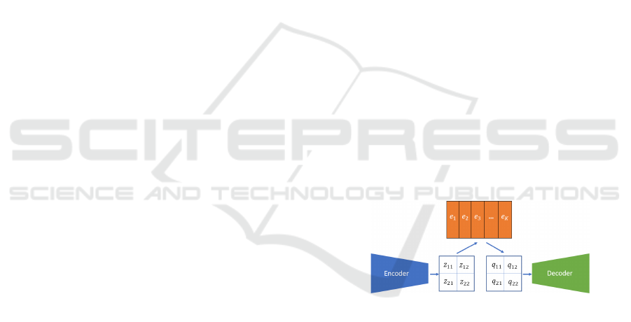
Figure 1: VQ-VAE (van den Oord et al., 2017) comprises
Encoder, VQ, and Decoder.
In the deep learning, a method for the vector quantiza-
tion of intermediate representations in each space or
time series was proposed in VQ-VAE (van den Oord
et al., 2017). In general, an autoencoder consists of
an encoder that outputs an intermediate representa-
tion z from input x and a decoder that outputs x from
z. Thus, VQ-VAE is one of the autoencoders. An au-
toencoder is trained so that input x and output ˆx of
the decoder are equal. For example, VAE (Kingma
and Welling, 2014) assumes a normal distribution in
the intermediate representation. This allows the de-
coder to generate new data similar to the training data
from the ˆz sampled from the normal distribution. On
the other hand, VQ-VAE assumes K discrete repre-
sentation spaces (Figure 1), where K is the number of
SDMIS 2021 - Special Session on Super Distributed and Multi-agent Intelligent Systems
554

representaion vectors.
In VQ-VAE, the intermediate representation q ∈
R
D×H×W
is described in equation 1, where the dis-
crete space representation is e ∈ R
K×D
and the output
of the encoder is z(x) × H ×W .
q
i j
= e
k
where argmin
k
ke
k
− z(x)k
2
2
(1)
In addition, to feed the backpropagation to z(x), the
input to Decoder ˆq is applied with equation 2, where
sg is an operation that points to a stop gradient.
ˆq = sg [q − z(x)] + z(x) (2)
The loss function for learning these is provided the
equation 3, where L
T
(x) is a task T -dependent loss
function.
L = L
T
(x) + ksg [q] − z(x)k
2
2
+ kq − sg [z(x)]k
2
2
(3)
In VQ-VAE, L
T
(x) = kx − ˆxk
2
2
equalizes input x and
output ˆx.
2.3 Sinkhorn–Knopp for
Representation Learning
Unsupervised representation learning automatically
extracts features from unlabeled data. DeepCluster
(Caron et al., 2018) uses CNN models such as VGG
(Simonyan and Zisserman, 2014) and ResNet (He
et al., 2016) to extract good features from images
that are well represented and easy to transfer to other
tasks. It is trained in three different steps as follows.
1. Transferring D-dimensional features to each im-
age by CNN
2. Clustering by K-means (Hartigan and Wong,
1979) based on the transferred feature
3. Training the model to predict to which cluster
each image belongs
Models trained by this method achieves then the state-
of-the-art in transition learning. On the other hand, a
problem inherent in the K-means-based method (and
as the assignment of the VQ-VAE (van den Oord
et al., 2017) is biased toward specific embedding vec-
tors) remains, i.e. the assignments are biased toward
a few specific clusters. For example, even if we wants
to assign images to 10,000 clusters, most images may
be assigned to dozens of clusters. This makes the
models to only a few rough clusters and prevented
them from learning more detailed information.
SeLa (YM. et al., 2020) is based on DeepCluster
but eliminates allocation bias among clusters by ap-
plying fast Sinkhorn–Knopp (Cuturi, 2013). When N
data are allocated to K clusters, SeLa performs an op-
timization using equation 4 as the objective function,
where P ∈ R
K×N
+
denotes the probability by model,
Q ∈ R
K×N
+
is targeted doubly stochastic matrix, U is
the set doubly stochastic matrix, and Q ∈ R
K×N
+
is the
double probability matrix such that the sum of each
row and each column is equal.
min
Q∈U
h
Q, −log P
i
+
1
λ
KL(QkQ) (4)
The first term of equation 4 minimizes the cross-
entropy distance between the predicted P and the tar-
get, and the second term constrains the distance be-
tween the equal double probability matrix Q and the
target so that it becomes small.
The fast Sinkhorn–Knopp (Cuturi, 2013) algo-
rithm optimizes Q based on equation 5.
Q = diag(α)P
λ
diag(β) (5)
λ is a hyperparameter that adjusts the first and second
terms of expression 4, and α, β are obtained using the
following progressive formulas:
∀y : α
y
← [P
λ
β]
−1
y
∀i : β
i
← [α
T
P
λ
]
−1
i
We can perform these iterative optimizations in high-
speed by using matrix operations and using the GPU.
2.4 Gradient Penalty
Gradient penalty has been proposed in DoubleBack-
propagation (Drucker and Le Cun, 1992). Recently,
Gradient penalty is used in generative deep learning
systems, such as WGAN-GP (Gulrajani et al., 2017)
to satisfy the 1-Lipschitz constant (smoothness of the
change in the output to the change in the input). In
this method, the equation 6 denotes the loss, where
C(x) is the function we want to vary smoothly and
5
x
refers to the derivative of the input x.
L
GP
(x) =
h
k
5
x
C(x)
k
2
2
− 1
i
2
(6)
In WGAN-GP, x is the alpha-blended image of the
training and generated data, and C(x) is the discrimi-
nator output.
On the other hand, DUO (Van Amersfoort et al.,
2020) introduces a gradient penalty for the input x
in addition to the usual CrossEntropyLoss implement
out-of-distribution detection, which detects objects
not included in the training data in the image clas-
sification tasks.
C(x) =
∑
y
exp
"
−
1
n
kW
y
f
θ
(x) − e
y
k
2
2
2σ
2
#
(7)
Vector Quantization to Visualize the Detection Process
555

In equation 7, y is the class label, f
θ
is the output of
the last layer of the model, W
y
is the class-specific
transfer matrix, e
y
is the embedding of the features of
each class, and σ is the hyperparameter for scaling.
Thus, adding the gradient penalty prevents excessive
changes in the loss function of the classifications ow-
ing to changes in the input. In other words, the effect
is such that the priority is to prevent a large change
in the loss function when a small change in the data
occurs, rather than to reduce the loss function for a
given data. This loss function allows the classifier to
react only to in-distribution data and not to out-of-
distribution data.
3 METHOD
3.1 VQ with Momentum
Sinkhorn–Knopp
VQ assigns the intermediate layer to the nearest em-
bedding space, and this assignment causes a problem
that the initial assignment bias affects the final learned
assignment to a specific embedding. In order to solve
this problem, we introduce Sinkhorn–Knopp (Cuturi,
2013), as used in SeLa (YM. et al., 2020). This en-
ables us to learn embedding to minimize the cost of
assigning to embedding space while increasing the as-
signment entropy of the selected embedding.
Let SK(P) be the embedding selected by
Sinkhorn–Knopp algorithm for the assignment prob-
ability P. Then, the expression for generating the em-
bedding corresponding to the output z(x) of the en-
coder can be written as equation 8 using the tempera-
ture parameter z(x).
q
i j
= e
k
where
SK(exp(−λke
k
− z(x)k
2
2
)) training
argmin
k
ke
k
− z(x)k
2
2
otherwise
(8)
In the case of SeLa (YM. et al., 2020), however, the
assignment is applied to the entire dataset in such a
way that it is equalized, but in order to apply it to
the intermediate layer, it is necessary to perform the
calculation for each batch. This is inefficient. There-
fore, we propose momentum Sinkhorn–Knopp. We
use α
t
and β
t
, which are moving averages of α and β
obtained from previous batches in iteration t, to use
expression 5 for each batch.
∀y : α
y
← [P
λ
β
t−1
]
−1
y
α
t
← (1 − m) × α + m × α
t
∀i : β
i
← [α
T
t
P
λ
]
−1
i
β
t
← (1 − m) × β + m × β
t
where m is an update parameter (m = 0.999 in this
study). This allows us to apply the Sinkhorn–Knopp
algorithm on a batch-by-batch basis, referring to pre-
vious batch assignments in high-speed.
3.2 Constant Embedding Space
VQ updates the discrete space representation (3), but
this changes the distance between each vector. In
this case, even if the Sinkhorn–Knopp algorithm can
achieve equal assignment to vectors, the similarity
problem in the vector representation may arise, re-
sulting in the same problem, i.e., the lack of equal
assignment. In order to improve the interpretability of
the intermediate representation, the distance between
each vector should be constant.
We propose constant embedding space, which
fixes the embedding space at the initial value sam-
pled from a normal distribution and does not update it
by learning. This technique makes it easy to perform
post-learning comparisons and solves the problem of
the similarity of the expressions.
3.3 Gradient Penalty
VQ with Sinkhorn–Knopp assignment and constant
embedding space improves the interpretability of in-
termediate representations, but this method has a neg-
ative effect on accuracy as shown in Table 1. The rea-
son why the accuracy decreased is that this method
increases the distance between embedding e
k
and en-
coder output z(x), and thus, makes the backpropaga-
tion not properly transmitted to the layers shallower
than the VQ.
Therefore, we add the following loss function to
the assignment of the embedding space as shown in
DUO (Van Amersfoort et al., 2020).
C(z) =
K
∑
k=1
exp
"
−
1
K
kz − e
k
k
2
2
2σ
2
#
(9)
This loss function prevents the cost of assignment to
the embedding space from overreacting to changes in
the input.
SDMIS 2021 - Special Session on Super Distributed and Multi-agent Intelligent Systems
556

4 EXPERIMENTAL RESULTS
In order to demonstrate the usefulness of the pro-
posed method, we have conducted two experiments.
The first one shows that the proposed method has a
similar classification accuracy compared with the one
without VQ and the assignment is more uniform than
that of the normal VQ. The second experiment shows
that embedding obtained using SK-VQ is more inter-
pretable than that of the normal VQ.
4.1 Accuracy and Assignment Entropy
We have measured how the classification accuracy
rate changes when applying VQ and the proposed
method to the intermediate layer of the classifica-
tion model, and confirmed its improvement compared
with the original model. Moreover, we show the mo-
mentum Sinkhorn–Knopp and constant embedding
increases the assignment entropy, which indicates the
uniformity of the assignment to each vector. We show
our method is superior to the normal VQ.
We have employed CIFAR10 as the dataset. It
contains 50,000 training data and 10,000 test data
for 10 classes of images of size 32 × 32. Further-
more, we chose Wide-Resnet-28-2 (Zagoruyko and
Komodakis, 2016) as the base CNN model. We train
the model from scratch with minibatch size 256 for
1000 epochs. We have more details in the appendix.
When applying VQ to the intermediate layer, we
have applied batch normalization (Ioffe and Szegedy,
2015) into the previous layer of VQ to stabilize the
training because the values are fixed in a normal dis-
tribution in the constant embedding space.
We compare the results with and without VQ, con-
stant embedding space, Sinkhorn–Knopp, and gradi-
ent penalty loss (Table 1).
Table 1: Accuracy and Assignment Entropy.
VQ CE SK GP Accuracy Entropy
94.55
X X 92.46 2.280
X X X 92.83 5.316
X X X X 93.06 5.311
4.2 Reconstruction
To show that the interpretability of the vector repre-
sentation obtained using SK-VQ is better than that
of the normal VQ, we have trained a decoder to re-
cover the original image from the vector representa-
tion. This is because the high image reproduction rate
of the decoder indicates that embedding is a relevant
feature space. In form, it is similar to autoencoder
such as VQ-VAE (van den Oord et al., 2017), but uses
fixed weights for the encoder and only trains the de-
coder.
We have also conducted experiments on VQ and
SK-VQ-GP. Table 2 shows the restoration errors. The
experimental results show that the restoration error
of the proposed method is smaller than that of VQ.
Therefore we can conclude that the proposed method
has a better reproducibility rate than that of VQ.
Table 2: Reconstruction Error.
Model Reconstruction Error
VQ 0.2733
SK-VQ-GP(ours) 0.1862
5 DISCUSSION
5.1 VQ with Momentum
Sinkhorn–Knopp
As Table 1 shows, we have achieved more or less
uniform assignments to the vector space by apply-
ing momentum Sinkhorn–Knopp to VQ. This allows
us to obtain various representations without being af-
fected by the initial values. On the other hand, we
believe that the gradient transmitted to the pre-VQ
layers in backpropagation is adversely affected by the
fact that the assignment is no longer made to the near-
est Embedding. However, fine-tuning using VQ with-
out Sinkhorn–Knopp can provide comparable or even
better accuracy than with Sinkhorn–Knopp, with little
loss of the assignment balance.
5.2 Constant Embedding Sampled from
a Normal Distribution
By introducing constant embedding, we are able to
maintain the distance of each embedding constant.
Moreover, the features are sampled based on a nor-
mal distribution, which makes it easier to compare the
strength of each feature. On the other hand, a nor-
mal distribution is not necessarily suitable for a fea-
ture space. For example, one-hot features are easier
to interpret, even if it is harder to learn in practice. As
a future investigation, we have to verify what distri-
bution is the most appropriate for feature spaces.
Vector Quantization to Visualize the Detection Process
557

5.3 Improved Accuracy by Gradient
Penalty
As Table 1 shows, the gradient penalty reduces
the loss of accuracy based on the momentum
Sinkhorn–Knopp and constant embedding in VQ. On
the other hand, the introduction of gradient penalty
without momentum Sinkhorn–Knopp and constant
embedding did not change the accuracy of the VQ sig-
nificantly. These indicate that the accuracy owing to
larger gap between the embedding space and the in-
termediate representation z caused by constraints as-
signed to the embedding space. In order to achieve
a comparable accuracy for normal VQ with constant
embedding in place, we need a loss function or model
that reduces the embedding space and the gap be-
tween the intermediate representations without in-
creasing the classification loss.
6 FUTURE WORK
6.1 Importance of Basis for Judgment
Pertaining to Disaster-Relief Drones
Figure 2: Road collapse site.
If we can visualize WHERE and HOW regarding a
decision in an image-based task, the applicability to
evacuation guidance tasks of drones during disasters
would increases drastically. Image data during a dis-
aster, especially in the midst of a disaster rather than
after it, is very difficult to collect, and that difficulty
makes machine-learning-based methods less accurate
than those of other methods. Nonetheless, errors in
judgment easily lead to risks pertaining to human
lives.
In a situation like Figure 2, for example, a classi-
fier on-board of a drones have to determine whether
the evacuees can pass this road or not in an emer-
gency. However, considering the answer “The evac-
uees cannot pass this road,” it is not clear that the road
is considered impassable because the left side is col-
lapsed, or because the remaining road on the right
side is also dangerous to pass. Furthermore, even if
it judges the right side be unsafe, it is impossible for
a human operator to judge whether it is simply be-
cause of the existence of cracks, or it is expected to
collapse soon, or simply it misjudged. It is extremely
difficult to solve these problems by simply increasing
the accuracy, and there is a need to quickly provide
feedback to the evacuees based on for their decisions.
The proposed method will make it easy to visu-
ally confirm the evacuation route determined by the
unmanned aircraft on the spot by providing the evacu-
ation route and decision-making rationale to the evac-
uees and controllers. If the decision-making rationale
is inconsistent with the visual assessment results of
the evacuees, the evacuees can request that the deci-
sion be corrected in advance. In addition, the pre-
sentation of the basis for the judgment can provide a
psychological reassurance to the evacuees.
For disaster relief, where the urgency is high and
a single mistake can be fatal, it is very important to
show the basis for decision-making. In the future, we
would like to show that it can be applied to disaster
relief tasks.
6.2 Creating a Model with a Different
Basis for Judgment
As exemplified by AdaBoost (Schapire, 1999), en-
sembles that make a final decision based on major-
ity votes of multiple classifiers that follow different
decision-making criteria are important and powerful
methods. Considering the deployment of multiple
drones at a disaster site, a group of drones with mul-
tiple decision-making criteria is more robust than a
group of drones with the same criteria. However, with
the existing the deep learning technique, creating sep-
arate models based on decisions is difficult.
The proposed method allows us to assign the in-
termediate layer to the embedding space, which is
more interpretable by the VQ, which allows us to cre-
ate models considering different decision bases. Sup-
pose we create Model A with the proposed method
and then train Model B with the same architecture.
To separate the decision bases of Models A and B, we
can perform adversarial training so that the embed-
ding space of Model A cannot be inferred from the
intermediate layer of Model B. The aforementioned
procedure can be used to create an ensemble model
or a model with multiple agents complementing each
other.
SDMIS 2021 - Special Session on Super Distributed and Multi-agent Intelligent Systems
558

6.3 WHERE to Detect and HOW to
Detect by VQ
To clarify WHERE to detect and HOW to detect by
VQ, we can anticipate the following steps. First, we
extract embedding and corresponding image regions.
Then, we aggregate the image regions allocated to the
same embedding region and provide them a label by
finding the common denominator. Finally, by looking
at the wrong labels during the test, we can figure out
“for what the model mistook a region.” It is presumed
that the above steps can be used to clarify the basis for
decisions.
The correspondence between embedding and
“which region” is not shown in this study, but it can
be possible by applying existing region visualization
methods such as SmoothGrad (Smilkov et al., 2017).
However, compared with the existing methods, a tai-
lored method is required to reveal the subdivided re-
gions.
Moreover, determining common denominators
and providing labels to the regions need to be done
manually at present. However, it is difficult to present
a representative image other than the low allocation
cost to embedding; therefore, it is necessary to show
that this allocation cost is a reliable indicator.
7 CONCLUSIONS
This study aims to create an AI system that consid-
ers WHERE to detect and HOW to detect. Such a
system is necessary in situations where everything is
urgent and errors are fatal, i,e., disaster scenes. For
this raeson, we have proposed three methods for deep
learning CNN models, based on the idea that the in-
terpretability can be improved by applying VQ to the
intermediate layer. First, we proposed the momen-
tum Sinkhorn–Knopp VQ. This method solves the
bias problem in the embedding selection, which is
an inherent problem of VQ, and has better restora-
tion performance than the normal VQ. Moreover, we
have used Sinkhorn–Knopp on a per-batch basis for
fast calculation. Second, we showed the effectiveness
of constant embedding space. The intermediate rep-
resentation, fixed by a normal distribution, allows us
to transfer the intermediate layer into an interpretable
feature space. Third, we have showed that gradi-
ent penalty improves the performance of momentum
Sinkhorn–Knopp and constant embedding space ap-
plied models. These proposed methods help us to re-
alize the first step to create a model that reveals how
to detect using VQ. Currently, we are planning to cre-
ate a method for visual decision-making and to cre-
ate a model with multiple decision-making bases. It
should be applied to and should be useful for disaster
relief activities.
ACKNOWLEDGMENTS
This work is supported in part by Japan Society for
Promotion of Science (JSPS), with the basic research
program (C) (No.17K01342), Grantin-Aid for Scien-
tific Research.
REFERENCES
Caron, M., Bojanowski, P., Joulin, A., and Douze, M.
(2018). Deep clustering for unsupervised learning of
visual features. In Ferrari, V., Hebert, M., Sminchis-
escu, C., and Weiss, Y., editors, ECCV (14), volume
11218 of Lecture Notes in Computer Science, pages
139–156. Springer.
Cubuk, E. D., Zoph, B., Shlens, J., and Le, Q. V. (2020).
Randaugment: Practical automated data augmentation
with a reduced search space. In 2020 IEEE/CVF Con-
ference on Computer Vision and Pattern Recognition
Workshops (CVPRW), pages 3008–3017.
Cuturi, M. (2013). Sinkhorn distances: Lightspeed compu-
tation of optimal transport. In Burges, C. J. C., Bot-
tou, L., Welling, M., Ghahramani, Z., and Weinberger,
K. Q., editors, Advances in Neural Information Pro-
cessing Systems, volume 26, pages 2292–2300. Cur-
ran Associates, Inc.
Drucker, H. and Le Cun, Y. (1992). Improving gener-
alization performance using double backpropagation.
IEEE Transactions on Neural Networks, 3(6):991–
997.
Goto, H., Ohta, A., Matsuzawa, T., Takimoto, M., Kam-
bayashi, Y., and Takeda., M. (2016). A guidance sys-
tem for wide-area complex disaster evacuation based
on ant colony optimization. In Proceedings of the 8th
International Conference on Agents and Artificial In-
telligence - Volume 1: ICAART,, pages 262–268. IN-
STICC, SciTePress.
Gulrajani, I., Ahmed, F., Arjovsky, M., Dumoulin, V., and
Courville, A. C. (2017). Improved training of wasser-
stein gans. In Guyon, I., Luxburg, U. V., Bengio, S.,
Wallach, H., Fergus, R., Vishwanathan, S., and Gar-
nett, R., editors, Advances in Neural Information Pro-
cessing Systems, volume 30, pages 5767–5777. Cur-
ran Associates, Inc.
Hartigan, J. A. and Wong, M. A. (1979). A k-means cluster-
ing algorithm. JSTOR: Applied Statistics, 28(1):100–
108.
He, K., Zhang, X., Ren, S., and Sun, J. (2016). Deep resid-
ual learning for image recognition. 2016 IEEE Con-
ference on Computer Vision and Pattern Recognition
(CVPR), pages 770–778.
Ioffe, S. and Szegedy, C. (2015). Batch normalization:
Accelerating deep network training by reducing in-
Vector Quantization to Visualize the Detection Process
559

ternal covariate shift. volume 37 of Proceedings of
Machine Learning Research, pages 448–456, Lille,
France. PMLR.
Kingma, D. P. and Welling, M. (2014). Auto-encoding
variational bayes. In 2nd International Conference
on Learning Representations, ICLR 2014, Banff, AB,
Canada, April 14-16, 2014, Conference Track Pro-
ceedings, volume abs/1312.6114.
Krizhevsky, A., Sutskever, I., and Hinton, G. E. (2012).
Imagenet classification with deep convolutional neu-
ral networks. In Pereira, F., Burges, C. J. C., Bottou,
L., and Weinberger, K. Q., editors, Advances in Neu-
ral Information Processing Systems, volume 25, pages
1097–1105. Curran Associates, Inc.
Liu, L., Jiang, H., He, P., Chen, W., Liu, X., Gao, J.,
and Han, J. (2020). On the variance of the adap-
tive learning rate and beyond. In International Con-
ference on Learning Representations, ICLR 2020,
https://openreview.net/forum?id=rkgz2aEKDr.
Ribeiro, M. T., Singh, S., and Guestrin, C. (2016). ”why
should I trust you?”: Explaining the predictions of any
classifier. In Proceedings of the 22nd ACM SIGKDD
International Conference on Knowledge Discovery
and Data Mining, San Francisco, CA, USA, August
13-17, 2016, pages 1135–1144.
Schapire, R. E. (1999). A brief introduction to boosting.
In Proceedings of the 16th International Joint Confer-
ence on Artificial Intelligence - Volume 2, IJCAI’99,
pages 1401–1406, San Francisco, CA, USA. Morgan
Kaufmann Publishers Inc.
Selvaraju, R. R., Cogswell, M., Das, A., Vedantam, R.,
Parikh, D., and Batra, D. (2017). Grad-cam: Visual
explanations from deep networks via gradient-based
localization. In Proceedings of the IEEE International
Conference on Computer Vision (ICCV), pages 618–
626.
Simonyan, K. and Zisserman, A. (2014). Very deep con-
volutional networks for large-scale image recognition.
CoRR, abs/1409.1556.
Smilkov, D., Thorat, N., Kim, B., Vi
´
egas, F., and Watten-
berg, M. (2017). Smoothgrad: removing noise by
adding noise. ArXiv, abs/1706.03825.
Taga, S., Tomofumi, M., Takimoto, M., and Kambayashi, Y.
(2019). Multi-agent base evacuation support system
using manet. Vietnam Journal of Computer Science,
06(02):177–191.
Tan, M. and Le, Q. (2019). EfficientNet: Rethinking model
scaling for convolutional neural networks. volume 97
of Proceedings of Machine Learning Research, pages
6105–6114, Long Beach, California, USA. PMLR.
Van Amersfoort, J., Smith, L., Teh, Y. W., and Gal, Y.
(2020). Uncertainty estimation using a single deep de-
terministic neural network. In III, H. D. and Singh, A.,
editors, Proceedings of the 37th International Con-
ference on Machine Learning, volume 119 of Pro-
ceedings of Machine Learning Research, pages 9690–
9700, Virtual. PMLR.
van den Oord, A., Vinyals, O., and kavukcuoglu, k. (2017).
Neural discrete representation learning. In Guyon,
I., Luxburg, U. V., Bengio, S., Wallach, H., Fer-
gus, R., Vishwanathan, S., and Garnett, R., editors,
Advances in Neural Information Processing Systems,
volume 30, pages 6306–6315. Curran Associates, Inc.
YM., A., C., R., and A., V. (2020). Self-labelling via simul-
taneous clustering and representation learning. In In-
ternational Conference on Learning Representations,
ICLR 2020, https://openreview.net/forum?id=Hyx-
jyBFPr.
Zagoruyko, S. and Komodakis, N. (2016). Wide residual
networks. In Richard C. Wilson, E. R. H. and Smith,
W. A. P., editors, Proceedings of the British Ma-
chine Vision Conference (BMVC), pages 87.1–87.12.
BMVA Press.
Zeiler, M. D. and Fergus, R. (2014). Visualizing and under-
standing convolutional networks. In Fleet, D., Pajdla,
T., Schiele, B., and Tuytelaars, T., editors, Computer
Vision – ECCV 2014, pages 818–833, Cham. Springer
International Publishing.
Zhang, M., Lucas, J., Ba, J., and Hinton, G. E. (2019).
Lookahead optimizer: k steps forward, 1 step back.
In Wallach, H., Larochelle, H., Beygelzimer, A.,
d'Alch
´
e-Buc, F., Fox, E., and Garnett, R., editors,
Advances in Neural Information Processing Systems,
volume 32, pages 9597–9608. Curran Associates, Inc.
Zhao, H., Jia, J., and Koltun, V. (2020). Exploring self-
attention for image recognition. In Proceedings of the
IEEE/CVF Conference on Computer Vision and Pat-
tern Recognition (CVPR), pages 10076–10085.
APPENDIX
Architecture. Our classification model architecture
is based on the stacking of residual blocks like Wide
Resnet (Zagoruyko and Komodakis, 2016), and the
application of VQ and batch normalization (Ioffe and
Szegedy, 2015) like Table 3. We set N = 28, k = 2,
and made the embedding space contain 256 embed-
dings.
Table 3: Classifier Architecture.
Group name Output size Block type
conv1 32 × 32 [3 × 3, 16]
conv2 32 × 32
3 × 3, 16 × k
3 × 3, 16 × k
× N
conv3 16 × 16
3 × 3, 32 × k
3 × 3, 32 × k
× N
conv4 8 × 8
3 × 3, 64 × k
3 × 3, 64 × k
× N
bn 8 × 8 [1 × 1]
vq 8 × 8 [1 × 1]
avg-pool 1 × 1 [8 × 8]
Moreover, we have designed a decoder to reproduce
the original image from the embedding of the classi-
fier, symmetrical with the Classifier (Table 4).
SDMIS 2021 - Special Session on Super Distributed and Multi-agent Intelligent Systems
560
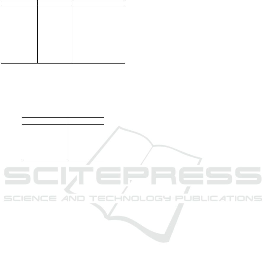
Table 4: Decoder Architecture.
Group name Output size Block type
conv1 8 × 8
3 × 3, 64 × k
3 × 3, 64 × k
× N
conv2 16 × 16
3 × 3, 32 × k
3 × 3, 32 × k
× N
conv3 32 × 32
3 × 3, 16 × k
3 × 3, 16 × k
× N
conv4
32 × 32 [3 × 3, 16]
conv5 32 × 32 [1 × 1, 3]
Training Details. We have used the Ranger Opti-
mizer, consisting of a composite of RAdam (Liu et al.,
2020) and Lookahead (Zhang et al., 2019). The hy-
perparameters are listed in Table 5.
Table 5: Optimizer Hyperparameters.
Parameter name Value
learning rate 1.0e
−3
weight decay 5.0e
−4
alpha 0.5
betas (0.95, 0.999)
eps 1.0e
−5
Moreover, we apply RandAugment (Cubuk et al.,
2020) for data augmentation. This allows generic data
augmentation for image classification to be adjusted
with a single parameter magnitude, which is one of
the standard data augmentation methods. Although
magnitude is magnitudein ∈ [0, 10], in this study, it is
adjusted with magnitude = 5.
Vector Quantization to Visualize the Detection Process
561
