
Hybrid Energy Production Analysis and Modelling for Radio Access
Network Supply
Greta Vallero
a
and Michela Meo
b
Department of Electronics and Telecommunications, Politecnico di Torino, Italy
Keywords:
Renewable Energy Sources, Wind Turbine, PV Panel, Radio Access Network, Base Station, Hybrid Power
Supply System, Modelling.
Abstract:
To move towards sustainability, Renewable Energy Sources (RES) have started to partially substitute fossil
fuels based energy generation. Also for the Information and Communication Technology (ICT) ecosystem
supply, and in particular in the Radio Access Networks (RANs), the usage of PV panels has been considered
an effective solution. Since the communication infrastructure has to be powered continuously, to face the
problem of the absence of the Photovoltaic (PV) panel energy production during the night, we consider a hybrid
solution, composed by a PV panel and a wind turbine, for the supply of Base Stations (BSs). Starting from
the characterisation of wind energy production, we assess the impact of the employment of the combination
of these RES on the excesses and deficits of energy production, highlighting that the hybrid solution better
fits the BS energy demand. In order to predict performance, we build polynomial models, which highlight the
effects of the variation of the installed wind and solar capacities.
1 INTRODUCTION
In order to comply with the Paris Agreement and the
European Green Deal, the electricity system has be-
gun a transition towards a more sustainable produc-
tion process (Commission, 2019). As a result, the
production share of fossil fuels has started reducing,
while a large RES penetration has been planned in
the next years. This is the response to achieve climate
goals, while facing the growth of the electricity de-
mand, which is supposed to maintain, until 2040, its
current increasing rate of 2.1% per year (IEA, 2020).
Besides the sustainability issues, this transformation
is also motivated by the petrol shock crisis, which will
occur at the end of the ”post-peak” period, in which
we are entering (Hirsch, 2008). This ”post-peak” pe-
riod starts after the peak oil moment, which occurs
at the maximum oil production phase. After this, the
oil production declines, causing energy price growth
and important economical implications. As a result,
in 2019, renewable electricity generation rose by 6%,
and 64% of this 6% derived from the installation of
new wind turbines and solar energy generators, which
are supposed to be further expanded to reach half of
a
https://orcid.org/0000-0002-6420-231X
b
https://orcid.org/0000-0001-7403-6266
the electricity generation by 2030 (IEA, 2020). Also
the supply of the ICT sector, responsible for 3% of the
CO
2
emissions in 2018 and, according to forecasts,
up to 14% in 2040, has been involved in this transfor-
mation (Belkhir and Elmeligi, 2018). The European
Commission, in (Bertoldi, 2017), under the need for
actions to improve the energy efficiency in commu-
nications, has formalised a policy for the regulation
of the energy consumption and the carbon emissions
of the Broadband Communication Equipment. Mean-
while, the communication community has recognised
the network energy efficiency as a fundamental and
urgent aspect. As well known, the BSs have been
identified as the most energy consuming components
of mobile networks (Gati et al., 2019), accounting for
80% of the total energy consumption of the Radio Ac-
cess Networks (RANs). The BSs energy consump-
tion is expected to further grow because of the rise of
the mobile IP traffic, which will reach 77.5 exabyte
(EB) per month by 2022 and 5 016 EB per month in
2030 (Gati et al., 2019; Forecast, 2019; Tariq et al.,
2020), more than, respectively, 6 and 400 times larger
than 11.5 EB per month occurred in 2017. To ad-
dress these issues, the usage of PV panel systems for
the supply of BSs, installed in proximity to these in-
frastructures, has been becoming an attractive solu-
tion (Chamola and Sikdar, 2016; Hassan et al., 2013;
Vallero, G. and Meo, M.
Hybrid Energy Production Analysis and Modelling for Radio Access Network Supply.
DOI: 10.5220/0010423601310141
In Proceedings of the 10th International Conference on Smart Cities and Green ICT Systems (SMARTGREENS 2021), pages 131-141
ISBN: 978-989-758-512-8
Copyright
c
2021 by SCITEPRESS – Science and Technology Publications, Lda. All rights reserved
131
Han and Ansari, 2014; Deruyck et al., 2017). Indeed,
besides the improvement of the RAN sustainability, it
is a promising approach to make the network more
independent from the power grid, as well as to re-
duce the network electricity bill, which is the key con-
tributor for the increase of the Operational Expendi-
ture (OPEX) (Renga and Meo, 2019; Pompili et al.,
2016). Because of this, 390 000 newly solar powered
BSs have been installed worldwide since 2012, at an
annual rate of 84 000 solar powered BS per year, 6
times higher with respect to 2012 and their usage is
expected to significantly advance in 6G RANs (Res.,
2013; Smertnik et al., 2014; Tariq et al., 2020). The
authors of (Deruyck et al., 2017) and (Aktar et al.,
2018) consider a PV panel system to reduce the CO
2
emissions used to generate energy by burning fossil
fuels, when powering a RAN; in (Guo et al., 2019) a
wind turbine system is considered for the same pur-
pose.
While the solution is promising, various issues
need to be addressed, among which the solar panel
dimensioning and the possible lack of energy gener-
ation due to its intermittent nature. Indeed, the so-
lar energy harvesting presents, as other RESs, ran-
domness, dependence on the weather conditions and
daily and seasonal variability, making these BSs
self-survival unstable. To tackle these issues, it is
fundamental to combine different renewable energy
sources. In this work, we consider the combination of
wind and solar RES for the supply of a BS, so as to
exploit their operating characteristics and to achieve
higher efficiency than the one that could be obtained
from a single energy source. In particular, in the first
part of our work, we analyse a data-set, which reports
real data of the energy production of wind turbines
and PV panel systems, installed in Belgium. Then,
we simulate a single BS, powered by an hybrid sys-
tem, composed by a PV panel and a wind turbine, us-
ing real mobile traffic demand and energy production
data. This scenario is evaluated in terms of energy
performance, expressed as annual bought energy and
annual wasted energy. Finally, models for the pre-
diction of this energy performance are proposed, as a
function of the installed capacity of the wind and so-
lar energy generators, in order to properly design the
energy system for future RANs.
2 DATA SET
In this work, we use the energy production data
provided by the Open Power System Data (OPSD)
project (Data, 2020). This data-set contains differ-
ent kinds of time series, such as onshore and off-
01:00 05:00 09:00 13:00 17:00 21:00
0.1
0.5
[Wh]
Typical day per each month
Solar En. Wind En.
Jan
Feb
Mar
Apr
May
Jun
July
Aug
Sept
Oct
Nov
Dec
(a)
0 2000 4000 6000 8000
ℓ
0.0
0.5
1.0
Dummy
ℓ=24 ℓ=365x24
Normalised R
X,X
(ℓ)
Solar En. Wind En.
(b)
0.1 0.3 0.5 0.7 0.9
Hourly Energy Production (Wh)
0.0
0.5
1.0
Dummy
Cumulative Density Function
Nightly Wind En.
Nightly Solar En.
Daily Wind En.
Daily Solar En.
(c)
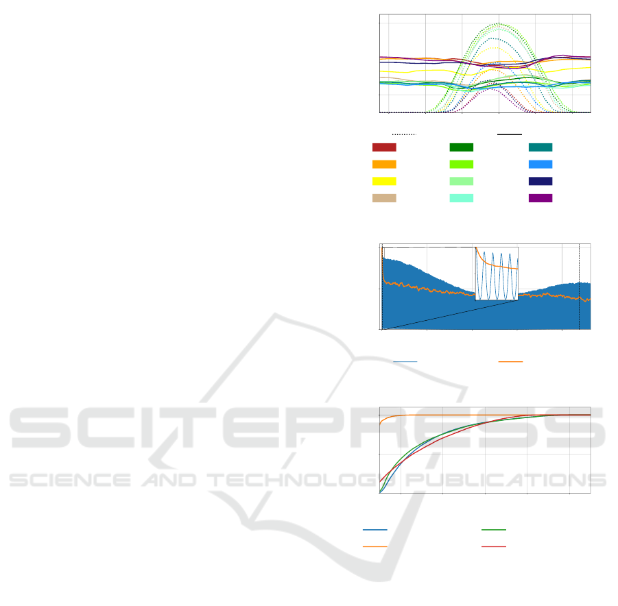
Figure 1: Characterisation of the Belgian wind and solar
energy production: (a) Daily wind and solar energy produc-
tion in each month, (b) Normalised Auto-correlation func-
tion R
X,X
(`) of the wind and solar energy production, (c)
Cumulative Density Function of the daily and nightly wind
and solar energy production.
shore wind power generation, solar power genera-
tion, installed wind and solar capacities, electricity
prices and electricity consumption, for 37 European
countries from 2012 to 2017. All variables are pro-
vided in hourly resolution, but some of them are also
available in higher resolution (half-hourly or quarter-
hourly). The data-set has been created by download-
ing the data of interest from the sources, i.e, from the
Transmission System Operators (TSOs) of the differ-
ent countries, resampling and merging them in a large
CSV file.
SMARTGREENS 2021 - 10th International Conference on Smart Cities and Green ICT Systems
132
Because of lack of some data, we select data from
01/01/2015 to 31/12/2017 of Belgium, Switzerland,
Germany and Denmark with hourly granularity and
we consider the actual wind energy production on-
shore, actual solar power production, wind moni-
tored capacity and solar monitored capacity fields,
which are reported in MW. Each production data is
normalised by the corresponding monitored capacity,
in order to compute the wind and solar power, in W,
which is produced by, respectively, a turbine and PV
panel system whose capacity is 1 W. Then, the hourly
energy produced by a wind/solar capacity of 1 W is
computed, in W h.
3 WIND ENERGY PRODUCTION
DATA
In this section, we discuss the characterisation of the
Belgian wind energy production as derived from the
used data-set. As mentioned in Sec. 2, it collects the
wind energy production, as well as the solar one, and
their corresponding installed capacity, registered be-
tween 2015 and 2017. We use these data to highlight
similarities and differences between solar and wind
energy production. In Fig. 1a, the typical energy pro-
duction day in each month is plotted. In particular,
plain and dashed lines indicate the mean hourly wind
and solar production, respectively, for each month.
First, we notice that, as largely discussed in (Hadji
et al., 2018; Renga et al., 2018), the solar generation
strictly depends on the presence of the sun. As a con-
sequence, a PV panel system produces energy only
for a limited amount of hours, which significantly
varies with the seasons, from 18 hours in June to 9
hours in December. This does not occur for the wind
energy: results suggest that a wind turbine system
produces for the whole duration of the day and its pro-
duction is almost constant during the day. Moreover,
the solar energy production peaks are much larger
in summer than in winter: they are around 0.5Wh
in May, when the maximum is reached, while no
larger than 0.13 Wh in December, corresponding to
the minimum peak, resulting in a drop by 73%. Quite
the opposite occurs for the wind energy production:
January, February, November and December, respec-
tively, in red, orange, blue and purple in the figure,
present the largest values for the wind energy produc-
tion.
The auto-correlation functions R
X,X
(`) of the solar
and wind energy production are reported in Fig. 1b,
in blue and orange, respectively. From this figure, it
is evident that the solar energy production is charac-
terised by a daily periodicity (see blue curve in the
2 3 4 5 6 7 8 9 10 11 12
K
0.0
0.2
0.4
Silhouette
0
200
400
SSE
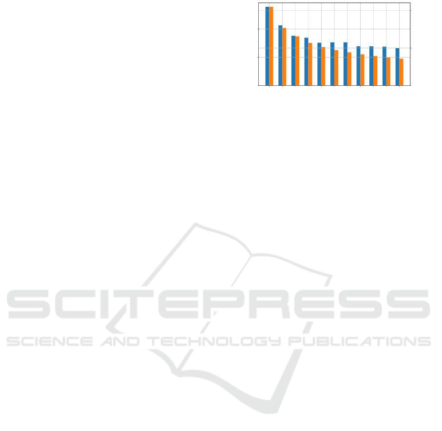
Figure 2: Silhouette index (left-y-axis, in blue) and SSE
index (right-y-axis, in orange) for different values of K.
zooming rectangle of Fig. 1b), as indicated by the vis-
ible peaks when ` of the auto-correlation is 24 or a
multiple of it. The presence of the peak when ` is
8760 means the presence of a seasonal periodicity in
the pattern. These are not the cases of the wind energy
generation. The orange curve in the figure indicates
the absence of any periodicity in the pattern and sug-
gests the high level of randomness of the wind energy
production.
Fig. 1c shows the Cumulative Distribution Func-
tions (CDFs) of the hourly wind and solar energy
production during the day, i.e. from 8 a.m. to 8
p.m. and during the night, i.e. from 8 p.m. to 8
a.m.. The curves, which correspond to the daily and
nightly wind energy production and to the daily solar
production, are similar and reach 1 around 0.65 Wh.
Meanwhile, as indicated by the figure, the hourly so-
lar production during the night is always lower than
0.05 Wh. This highlights again the different variation
within the daily pattern, provided by the two energy
sources. Moreover, contrary to the hourly solar en-
ergy production, the hourly wind production is close
to zero with infinitesimal probability.
3.1 Clustering
In order to explore the daily wind energy production
and extract typical daily patterns, the K-means clus-
tering algorithm is employed. We consider as an ob-
servation the daily pattern of hourly wind energy gen-
eration; i.e., a vector of 24 elements where each ele-
ment is the energy production in a given hour of a day.
The K-means partitions the observations into K clus-
ters in which each observation belongs to the cluster
with the nearest mean, i.e. the nearest centroid, so as
to minimise the within-cluster variance. In particu-
lar, the K-means algorithm starts with K random cen-
troids, and then performs iterative calculations to op-
timise the positions of these centroids, until they sta-
bilise. In each iteration, the assignment step and the
update step are performed. In the assignment step,
each observation is assigned to the cluster with the
Hybrid Energy Production Analysis and Modelling for Radio Access Network Supply
133
Jan
Feb
Mar
Apr
May
Jun
July
Aug
Sept
Oct
Nov
Dec
0
10
N. days
Patterns in Cluster 0
(a)
Jan
Feb
Mar
Apr
May
Jun
July
Aug
Sept
Oct
Nov
Dec
0
10
N. days
Patterns in Cluster 1
(b)
Jan
Feb
Mar
Apr
May
Jun
July
Aug
Sept
Oct
Nov
Dec
0
10
N. days
Patterns in Cluster 2
(c)
Jan
Feb
Mar
Apr
May
Jun
July
Aug
Sept
Oct
Nov
Dec
0
10
N. days
Patterns in Cluster 3
(d)
Jan
Feb
Mar
Apr
May
Jun
July
Aug
Sept
Oct
Nov
Dec
0
10
N. days
Patterns in Cluster 4
(e)
01:00
05:00
09:00
13:00
17:00
21:00
0.0
0.5
[Wh]
Centroids
(f)
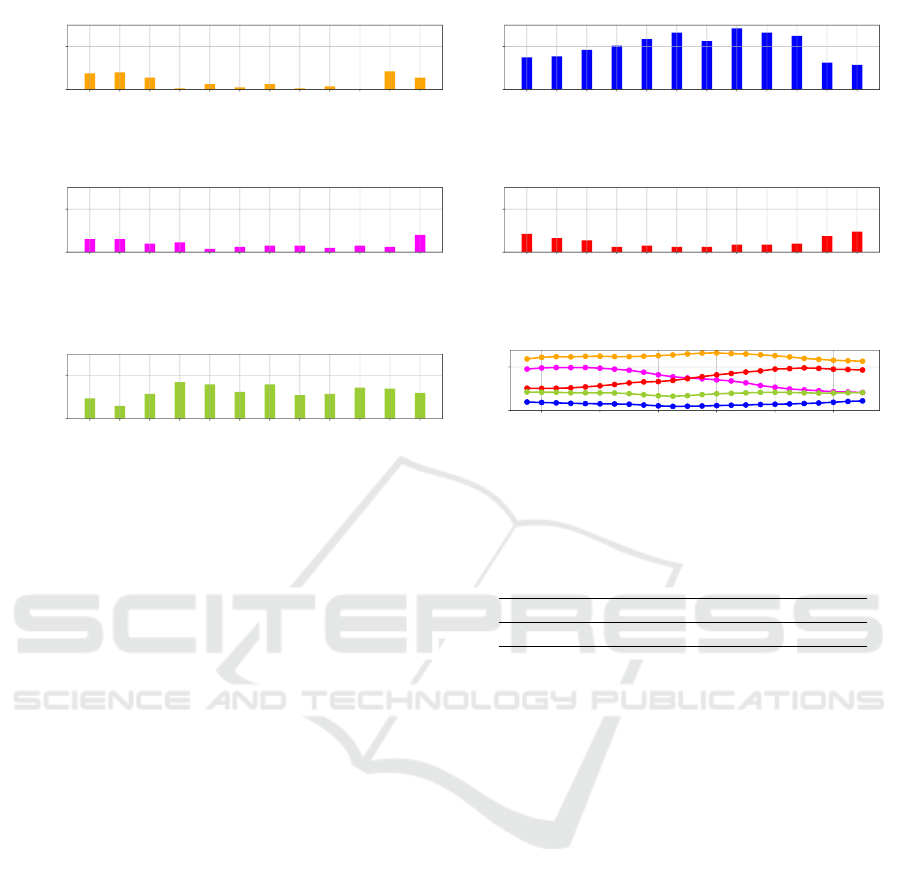
Figure 3: Results of the clustering with K=5: (a)-(e) number of observations clustered in each cluster, (f) resulting centroids.
nearest mean. The update step recalculates the cen-
troid of each cluster, as the mean of the observations
assigned to that cluster. Since the performance of the
algorithm depends on the random initialisation of the
centroids, the algorithm is performed 100 times with
different random seeds.
We perform this procedure for the numbers of
clusters K, varying between 2 and 12. Then, we select
the K solution, using the Elbow method (Bholowalia
and Kumar, 2014; Kodinariya and Makwana, 2013).
According to it, the optimal number of clusters is in-
dicated by the elbow of the curve of the Sum of the
Squared Error (SSE), or distortions, and of the Silhou-
ette parameter (Petrovic, 2006; Desgraupes, 2013).
The SSE is the sum of distance of each observation,
i.e., a daily wind energy production pattern in our
case, from the centroid of the cluster it belongs; the
Silhouette parameter provides a measure of how close
an observation is from its centroid, compared to the
distance from the others. Fig.2, where the Silhouette
and Distortion indexes are plotted in blue and orange,
respectively, indicates that the best choice for K is 5.
Figure 3 illustrates the results of the clustering with
K equals to 5. In particular, in Fig. 3f, each curve
corresponds to the centroid of each of the 5 clusters,
while Figs. 3a-3e report, for each cluster, the number
of daily patterns, in each month, assigned to the cor-
responding cluster; the colours of the distributions of
points in clusters are the same used for the centroids.
Fig. 3f highlights that the algorithm identifies a clus-
ter, characterised by a very low daily energy produc-
Table 1: Values of the parameters of the consumption model
for macro and small cell BSs.
BS type N
trx
P
max
(W) P
0
(W) ∆
p
Macro 6 20 84 2.8
tion, never larger than 0.12 Wh, (blue curve in the fig-
ure, corresponding to cluster 1) and another, plotted
in green in the figure (Cluster 4), when the produc-
tion is larger, between 0.17 and 0.22 Wh. Significant
higher values are reached by the centroids plotted in
yellow, red and pink. For these clusters, these large
production values, always larger than 0.22 Wh and up
to 0.66 Wh, are reached during the first part of the day
(see pink curve in Fig. 3f), in the last part, as for the
red curve in Fig. 3f, or for the whole duration of the
day (see yellow curve in Fig. 3f). From Figs. 3a-
3e, we notice that the largest part of patterns belong
to the clusters, whose centroid is characterised by the
lowest daily wind energy production (i.e. blue and
green curves in Fig. 3f). On the contrary, the clusters,
whose centroid reaches a large amount of produced
energy during part of the day (see pink and red curves
in Fig. 3f), or for the whole duration of the day (yel-
low curve in Fig. 3f), have few patterns and those
patterns occur typically during the winter months, i.e.
January, February, November and December, while
summer is characterised by low production levels.
SMARTGREENS 2021 - 10th International Conference on Smart Cities and Green ICT Systems
134

4 SIMULATION SET UP
In this part of the work, we consider a single macro
cell BS of a RAN, supplied by a hybrid system, with
total capacity C
tot
, in kW, composed by a wind tur-
bine, whose capacity is W , in kW, and a PV panel
system, with capacity S, in kW, and the grid. Data
provided by a large Italian mobile network operator
are used in this study. They report the traces of the
traffic demand volume, in bits, of numerous BSs lo-
cated in Milan, Italy, for two months in 2015, with
granularity of 15 minutes. The traffic traces are ag-
gregated to derive an hourly granularity and they are
averaged in order to obtain the typical daily traffic de-
mand of each BS, with an hourly granularity. For our
work, two different traces are selected, corresponding
to BSs, located in different areas of the city, in order
to consider samples of quite different scenarios, and,
hence, traffic patterns, which are representative of the
various zones that coexist in an urban environment.
First, a BS located in proximity of the train station
area is selected. It is characterised by intense activity
levels, especially at the beginning and at the end of the
working hours. The second BS is picked in the San
Siro district, which includes a large soccer stadium,
meaning that the activity here is variable depending
on the scheduled matches and concerts, resulting very
heavy when these events occur.
The input power required for the operation of a
BS in an hour, denoted as E
(t)
in
, in Wh, is derived ac-
cording to the linear model proposed in (Auer et al.,
2010):
E
(t)
in
= N
trx
· (P
0
+ ∆
p
P
max
ρ), 0 ≤ ρ ≤ 1 (1)
where N
trx
is the number of transceivers, P
0
represents
the power consumption when the radio frequency out-
put power is null, ∆
p
is the slope of the load dependent
power consumption, ρ is the traffic load and P
max
is
the maximum radio frequency output power at max-
imum load. Table 1 summarises the value of the pa-
rameters for a macro cell BSs (Auer et al., 2010).
As already mentioned, the considered BS is sup-
plied by an hybrid RES system, composed of a PV
panel and a wind turbine. The Belgian data for the
wind and solar energy, generated by, respectively, a
wind turbine and a PV panel, located in Belgium, are
used, taken from (Data, 2020) and presented in sec-
tion 2. As mentioned above, the data-set provides the
amount of Watt produced by a PV panel and a wind
turbine, both with capacity of 1 W. In order to derive
the energy generated by the simulated RES system,
we multiply these data by their capacity, expressed in
Watt.
In our simulations, we assume that each consid-
ered BS operates for 3 years. The BS uses the green
power generated by the RESs and when the energy
production exceeds the BS consumption, that amount
of energy is wasted. In case the generated energy is
not enough to power the BS, the missing energy is
bought from the grid. In each time slot, which lasts
1 hour, the BS energy consumption E
(t)
in
is computed,
as in (1), and, knowing the energy that is generated
by the supply system, E
(t)
pr
, during that time slot, the
bought and wasted energy are computed. The bought
energy E
(t)
b
measures the amount of energy, in Wh,
which is bought from the grid during that time slot,
when the RES system does not produce enough en-
ergy for the BS supply; the wasted energy E
(t)
w
pro-
vides the total energy, in Wh, which exceeds the BS
energy consumption and so it is not used. They are
given by:
E
(t)
b
= max (0, E
(t)
in
− E
(t)
pr
) (2)
E
(t)
w
= max (0, E
(t)
pr
− E
(t)
in
) (3)
where E
(t)
in
is the energy consumed at time t, computed
as in (1), E
(t)
pr
is the energy produced by the power
supply system at time t
Once a simulation is completed, the following en-
ergy metrics are computed:
• E
b
: it is the average amount of energy, measured
in Wh/year, which is bought from the grid every
year. It is computed as follows:
E
b
=
1
Y
Y ·365·24
∑
t=0
E
(t)
b
(4)
where E
(t)
b
is the energy bought from the grid at
time t, computed as in (2) and Y is the number of
considered years.
• E
b,h
: it accounts for the bought energy, in
Wh/year, at hour h, with h = 0, 1, 2, .., 23, in each
year. It is given by:
E
b,h
=
1
Y
Y ·365·24
∑
t=0
t%24=h
E
(t)
b
(5)
where, as above, E
(t)
b
is the energy bought from
the grid at time t (see (2)) and Y is the number of
considered years.
• E
w
: it provides the annual wasted energy, in
Wh/year:
E
w
=
1
Y
Y ·365·24
∑
t=0
E
(t)
w
(6)
where, E
(t)
w
is the wasted energy in time slot t, de-
rived as in (3) and Y is the number of considered
years.
Hybrid Energy Production Analysis and Modelling for Radio Access Network Supply
135

• E
w,h
: it measures the amount of wasted energy, in
Wh/year, at hour h, with h = 0, 1, 2, .., 23, in each
year. It is computed as:
E
w,h
=
1
Y
Y ·365·24
∑
t=0
t%24=h
E
(t)
w
(7)
where, as above, E
(t)
w
is the wasted energy at time
t, computed as in (3) and Y is the number of con-
sidered years.
5 SIMULATION RESULTS
In this section, we discuss the results of the simu-
lations, using the metrics presented above. Besides
the impact of the total installed RES capacity C
tot
on
these metrics, we also investigate the impact of its dis-
tribution between the PV panel capacity, S, and the
wind turbine capacity, W . In particular, we consider
C
tot
equal to 1 kW, 4 kW and 5 kW and we vary its
distribution among the solar and wind energy gen-
erator systems. The results are compared with our
benchmark, i.e., the scenario in which no RES is used
and the electricity needed for the BS supply is totally
taken from the grid. This means that E
b
is equal to
the annual BS energy consumption, which is, accord-
ing to our simulations, 5.1 MWh for San Siro BS and
5.6 MWh for the Train Station BS; E
w
is 0 MWh.
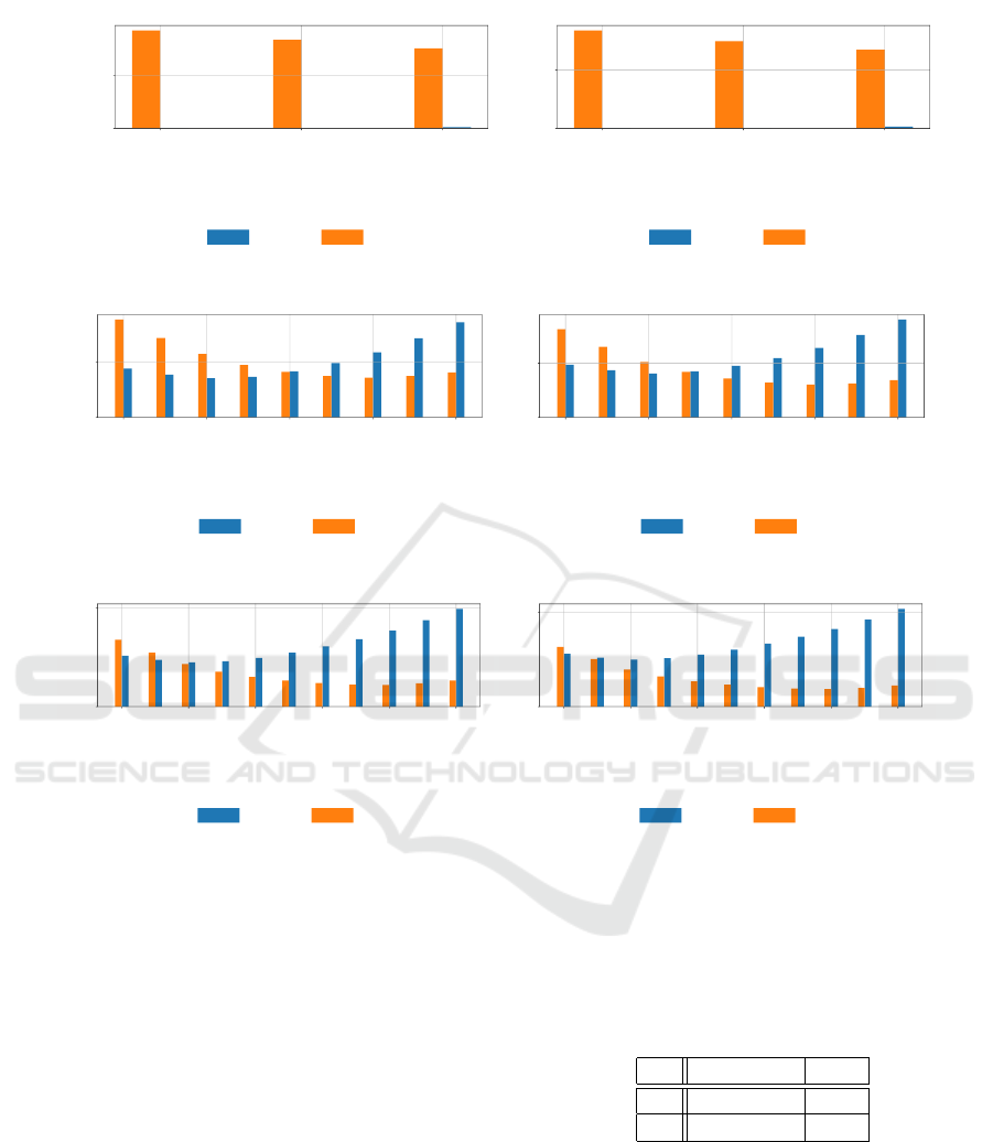
In Fig. 4, E
w
and E
b
, in blue and orange, respectively,
are plotted, for the Train Station BS, on the left, and
the San Siro BS, on the right. Each row of the fig-
ure considers different total RES installed capacity:
1 kW, in Figs. 4a, 4b, 4 kW in Figs. 4c, 4d and 5 kW
in Figs. 4e, 4f. On the left of each plot, only the so-
lar capacity is used, while moving towards right, so-
lar capacity diminishes by 0.5 kW and the capacity
of the wind turbine grows of 0.5 kW at each step,
i.e., at each group of bars. From Fig. 4, we first no-
tice that E
b
and E
w
significantly vary with different
C
tot
. Indeed, the energy bought from the grid, E
b
, de-
creases if the total capacity grows, from a maximum
of 5.56 MWh, when C
tot
is 1 kW, to a minimum of
0.93 MWh, when the capacity of RES is 5 kW. Sim-
ilarly, when the C
tot
becomes larger, the waisted en-
ergy, E
w
, rises, from 0 MWh, when C
tot
is 1 kW, to a
maximum of 4.97 MWh with C
tot
equals to 5 kW.
Results in Fig. 4 reveal that E
b
and E
w
are also af-
fected by the different distributions of these capacities
between the wind and solar systems. Indeed, given a
fixed total capacity C
tot
, if the portion of wind capac-
ity grows, E
b
decreases but E
w
increases. When C
tot
is
1 kW, the reduction of the E
b
is 17% and 18% with re-
spect to the chosen benchmark, in San Siro and Train
Station areas, respectively, if the capacity is totally
used as PV panel capacity. Meanwhile, E
b
reaches its
minimum value, dropping up to 34%, if all the capac-
ity is employed for the wind turbines. The situation is
different when C
tot
is larger. Indeed, when it is 4 kW,
for each considered BS, the minimum E
b
is reached
when the wind and the solar capacities are, respec-
tively, 3 kW and 1 kW. In this scenario, E
b
drops by
74% and 76%, for the BS in the Train Station and San
Siro areas, respectively. In this case, the annual E
w
is
1.43 MWh/year and 1.22 MWh/year, respectively.
Each curve in Fig. 5b represents E
w,h
, with
h = 1,2,...,24, i.e., the total amount of energy which
is wasted during a year at each hour of the day, for
the Train Station BS, for different W and S combina-
tions, given C
tot
equal to 4 kW. Values of E
w,h
close
to 0 MWh are given before 7.00 a.m. and after 7.00
p.m., for values of W lower than 1.5 kW, which im-
plies S larger than 2.5 kW (see light green, orange and
blue curves in Fig. 5b). This is because the PV panel
is not producing in these hours and the small capac-
ity of the wind turbine does not exceed in production
for the BS supply. Between 7.00 a.m. and 7.00 p.m.,
the PV panel produces energy because of the sun’s
presence. In this period of the day, the case with W
and S equal to 1.0 kW and 3.0 kW, respectively, pro-
vides the lowest E
w,h
, among the scenarios with W
and S, respectively, lower than 1.5 kW and larger than
2.5 kW. Quite the opposite occurs for E
b
,h, , with
h = 1,2,...,24, whose behaviour is plotted in Fig. 5a,
for different combinations of W and S, when C
tot
is
equal to 4 kW, for the Train Station BS. For values
of W larger than 2.5 kW and, consequently, S lower
than 1.5 kW, E
b,h
is no larger than 0.08 MWh, before
8.00 a.m. and after 6.00 p.m., as denoted by the pink,
grey and dark green curves in Fig. 5a. In the same
time interval, if W is lower than 2.5 kW and S larger
than 1.5 kW, E
b,h
increases up to z MWh. Between
8.00 a.m. and 6.00 p.m., because of the limited con-
tribution from the PV panel when its capacity is not
larger than 0.5 kW, E
b
,h grows up to 0.1 MWh, mak-
ing the scenario with solar and wind capacities equal
to 3.0 kW and 1.0 kW the best in terms of E
b
.
Nevertheless, as can be seen in Fig. 4c, if the tur-
bine has capacity 2.5 kW and the PV panel 1.5 kW,
the E
b
drops by 73% and 75% with respect to the
benchmark scenario, respectively, resulting therefore
slightly larger than the previous case, where, as men-
tioned, up to 74% and 76% of reduction is achieved.
Nevertheless, this reduces E
w
by 16% and 14%. Sim-
ilarly, when C
tot
is 5 kW, the hybrid solution, with
4 kW of wind capacity and 1 kW of solar one provides
the lowest amount of E
b
, as can be noticed in Figs. 4e
and 4f. It results no larger than 1.1 MWh/year, re-
SMARTGREENS 2021 - 10th International Conference on Smart Cities and Green ICT Systems
136
W:0.0
S:1.0
W:0.5
S:0.5
W:1.0
S:0.0
Installed capacity [kW]
0.0
2.5
MWh
Train Station with C
tot
: 1kW
E
w
E
b
(a)
W:0.0
S:1.0
W:0.5
S:0.5
W:1.0
S:0.0
Installed capacity [kW]
0.0
2.5
MWh
San Siro with C
tot
: 1kW
E
w
E
b
(b)
W:0.0
S:4.0
W:1.0
S:3.0
W:2.0
S:2.0
W:3.0
S:1.0
W:4.0
S:0.0
Installed capacity [kW]
0
2
MWh
Train Station with C
tot
: 4kW
E
w
E
b
(c)
W:0.0
S:4.0
W:1.0
S:3.0
W:2.0
S:2.0
W:3.0
S:1.0
W:4.0
S:0.0
Installed capacity [kW]
0
2
MWh
San Siro with C
tot
: 4kW
E
w
E
b
(d)
W:0.0
S:5.0
W:1.0
S:4.0
W:2.0
S:3.0
W:3.0
S:2.0
W:4.0
S:1.0
W:5.0
S:0.0
Installed capacity [kW]
0
5
MWh
Train Station with C
tot
: 5kW
E
w
E
b
(e)
W:0.0
S:5.0
W:1.0
S:4.0
W:2.0
S:3.0
W:3.0
S:2.0
W:4.0
S:1.0
W:5.0
S:0.0
Installed capacity [kW]
0
5
MWh
San Siro with C
tot
: 5kW
E
w
E
b
(f)
Figure 4: Simulations results: (a) E
b
and E
w
with C
tot
equal to 1 kW for the Tran Station BS, (b) E
b
and E
w
with C
tot
equal
to 1 kW for the San Siro BS (c) E
b
and E
w
with C
tot
equal to 4 kW for the Tran Station BS, (d) E
b
and E
w
with C
tot
equal to
4 kW for the San Siro BS, (e) E
b
and E
w
with C
tot
equal to 5 kW for the Tran Station BS, (f) E
b
and E
w
with C
tot
equal to
5 kW for the San Siro BS.
duced by more than 80% with respect to our bench-
mark, but with an amount of wasted energy larger
than 3.8 MWh/year. In order to reduce this by 26% for
the Train Station BS and by 19% for the San Siro one,
we employ a wind turbine with a capacity of 3 kW and
a PV panel, whose capacity is 2 kW, at the expense of
a little rise of the E
b
, still resulting lower than 76% of
E
b
in the benchmark scenario.
These results show that hybrid solutions reduce
both E
b
and E
w
. Indeed, for what concerns E
b
, the hy-
brid solution copes with the lack of energy production
by PV panel during the night, thanks to the turbine
production. Meanwhile, the employment of the PV
panel provides a large support to the BS supply dur-
ing the BS energy consumption peaks, which occur
Table 2: p-value for the energy performance metrics E
b
, E
w
and the different input parameters W and S.
E
b
E
w
W 0.0 0.0
S 3.0 ·10
−47
0.05
daily, during the PV panel generation periods. Focus-
ing on E
w
, the hybrid solutions avoid that the wind
turbine energy production exceeds the consumption
during the night, when the BS energy consumption
reaches its minimum. Similarly, the hybrid solution
prevents wasting energy during the day, during the PV
panel production hours.
Hybrid Energy Production Analysis and Modelling for Radio Access Network Supply
137

01:00
05:00
09:00
13:00
17:00
21:00
0.0
0.1
0.2
0.3
MWh
Train Station: E
b,h
with C
tot
: 4kW
W=0.0;S=4.0
W=0.5;S=3.5
W=1.0;S=3.0
W=1.5;S=2.5
W=2.0;S=2.0
W=2.5;S=1.5
W=3.0;S=1.0
W=3.5;S=0.5
W=4.0;S=0.0
(a)
01:00
05:00
09:00
13:00
17:00
21:00
0.0
0.1
0.2
0.3
MWh
Train Station: E
w,h
with C
tot
: 4kW
W=0.0;S=4.0
W=0.5;S=3.5
W=1.0;S=3.0
W=1.5;S=2.5
W=2.0;S=2.0
W=2.5;S=1.5
W=3.0;S=1.0
W=3.5;S=0.5
W=4.0;S=0.0
(b)
Figure 5: Simulation results for the Train Station BS, with C
tot
equal to 4 kW, varying its distribution between solar and wind
capacity: (a) E
b,h
, h=1,2,...,23 (b) E
w,h
, h=1,2,...,23.
Table 3: Coefficients of the models for the prediction of E
b
.
Country a
b
b
b
c
b
d
b
e
b
K
b
Belgium -831.33 -1582.29 0.09 0.10 0.16 5·10
6
Denmark -1697.26 -793.37 0.18 0.11 0.08 5.12·10
6
Germany -1617.87 -851.37 0.16 0.10 0.09 5.23·10
6
Switzerland -1525.72 -685.82 0.15 0.08 0.07 5.30·10
6
6 PREDICTION MODEL
In this section, we propose two analytical prediction
models to derive E
b
and E
w
, in different locations,
namely, Belgium, Denmark, Germany and Switzer-
land. These models are based on the relation between
E
b
, E
w
, in W h, and the installed wind and solar capac-
ity, W and S, in W . The aim of this model is to provide
a tool to investigate and predict the yearly bought and
wasted energy, when designing the RES system, for a
BS supply located in a given country.
First, for each country, we run multiple simula-
tions, as described in section 4, to create a data-set
used to build each model of each country. These sim-
ulations are performed with different values of W and
S and for each pair of values for W and S, two dif-
ferent simulations are performed, one considering the
traffic demand of the Train Station BS and the other
the traffic demand of the San Siro BS. For each simu-
lation, E
b
and E
w
are computed, so that a data-set for
E
b
and another for E
w
are built. Each row of the E
b
data-set contains the installed wind capacity W , the
installed solar capacity S and the resulting E
b
, when
these capacities are employed to power the considered
BS. Similarly, in each entry of the E
w
data-set, there
are the employed capacities W and S and the obtained
E
w
. First,the statistical significant relations between
W , S and our energy metrics E
b
and E
w
is verified.
To do this, we use the p-value index. The p-value
results for each country are reported in Table 2, pre-
senting each value lower or equal to 0.5, confirming
the existence of statistical relationships between these
parameters.
We model this relationship as a second degree
polynomial, as suggested by Fig. 4. For each coun-
try, receiving as input the solar and the wind capacity,
S and W , the values of E
b
and E
w
are computed as
follows:
E
b
= a
b
S + b
b
W + c
b
S
2
+ d
b
SW + e
b
W
2
+ K
b
(8)
E
w
= a
w
S + b
w
W + c
w
S
2
+ d
w
SW + e
w
W
2
(9)
where a
b
, b
b
, a
w
and b
w
are in W h/W , c
b
, d
b
, e
b
, c
w
,
d
w
and e
w
in W h/W
2
and K
b
in W h. Each coefficient
of each model is defined through the Linear Regres-
sion, using 66% of the corresponding data-set. The
remaining 34% is employed as a test set for the model
evaluation. Note that in the model of E
w
, the constant
term is not present, so that E
w
is 0 MWh, when C
tot
is
SMARTGREENS 2021 - 10th International Conference on Smart Cities and Green ICT Systems
138
Table 4: Coefficients of the models for the prediction of E
w
.
Country a
w
b
w
c
w
d
w
e
w
Belgium 57.05 100.29 0.11 0.15 0.18
Denmark -8.98 73.81 0.19 0.14 0.09
Germany -83.70 -8.04 0.17 0.12 0.09
Switzerland -56.00 -78.81 0.15 0.09 0.06
Table 5: R
2
and NMRSE of the models used for E
b
(R
2
b
and NMRSE
b
, respectively) and E
w
(R
2
w
and NMRSE
w
, respectively),
for each country.
Country R
2
b
NMRSE
b
R
2
w
NMRSE
w
Belgium 0.97 0.08 0.99 0.07
Denmark 0.97 0.08 0.99 0.07
Germany 0.98 0.07 0.99 0.08
Switzerland 0.97 0.07 0.99 0.10
0 kW.
The resulting coefficients for E
b
and E
w
models
are listed in Tables 3 and 4. In Table 5, each row re-
ports R
2
b
and NMRSE
b
, which are R
2
and NMRSE,
computed on the test set, for the model of each coun-
try, to predict E
b
. The table also gives R
2
and NMRSE
of the model for the E
w
prediction, respectively R
2
w
and NMRSE
w
. According to these values, these mod-
els predict E
b
and E
w
in at least 97% of the cases, as
indicated by R
2
always larger or equal to 0.97, with
an error never larger than 0.10.
The curve of models of E
b
and E
w
is shown in
Figs. 6a, 6b, 6c, 6d, and 6e, 6f, 6g, 6h in Bel-
gium, Denmark, Germany and Switzerland, respec-
tively. First, we notice that the resulting model of E
b
presents visible differences in Belgium with respect
to the other countries. Indeed, in Belgium, the growth
of the wind capacity W impacts more than the rise of
the solar capacity S, as can be seen in Fig. 6a. In
this model, the coefficients which multiply W , i.e., b
b
and e
b
, are larger, in absolute value, than, respectively
a
b
and c
b
, which multiply S, making E
b
more variable
when that input parameter grows or decreases (see Ta-
ble 3). Quite the opposite occurs for the other consid-
ered countries (see Figs. 6b, 6c and 6d). Indeed, in
these cases, as reported in Table 3, the absolute values
of b
b
is always lower than a
b
, as well as the one of e
b
is always smaller than the one of c
b
. This means that,
for these countries, the variation of S affects more E
b
than the W one. Similarly, for the E
w
model, as can
be seen in Table 4, e
w
is larger than c
w
, in the Bel-
gian case, making it more affected by the variation
of W than of S. Meanwhile, for the Danish, German
and Swiss cases, e
w
is lower than c
w
, meaning that the
grow or the drop of S impacts more E
w
that the varia-
tion of W .
In Figs. 7a, 7b, 7c and 7d, each curve is computed
with the E
b
model and represents E
b
for a given C
tot
,
increasing the installed solar capacity S, while dimin-
ishing the wind capacity W . We notice that, while the
Belgian case presents a growing trend (see 7a), for
the other countries the trend is decreasing, as can be
observed in Figs. 7b, 7c, 7d. This means that, accord-
ing to the used data, for the supply of a BS, the wind
capacity provides more usable energy than the solar,
in Belgium, while quite the opposite occurs in Den-
mark, Germany and Switzerland. From these figures,
we also notice that for C
tot
large enough (larger than
2 kW), the hybrid solution is convenient, in terms of
E
b
and E
w
, as in the simulation results, discussed in
section 5.
7 CONCLUSIONS
In order to make RANs more sustainable and reduce
the OPEX, a hybrid system, composed by a PV panel
and a wind turbine, is considered for the BS supply, in
addition to the electric grid. First, based on real data,
we characterise the Belgian wind energy production,
comparing it with the solar one. Results reveal that,
while the solar production presents significant differ-
ences between daily and nightly hours, the nightly and
daily wind generations are almost identical. More-
over, while the largest solar energy production occurs
in summer, quite the opposite occurs for the wind en-
ergy production, which reaches its maximum produc-
tion in winter. Hence, hybrid systems allow to better
follow the BS demand with respect to single source
systems. Indeed, simulation results reveal that the hy-
brid system supply provides significant reduction of
the energy which needs to be bought from the grid.
The presence of the turbine provides nightly energy
supply to satisfy the small BS energy demand dur-
Hybrid Energy Production Analysis and Modelling for Radio Access Network Supply
139

S [kW]
0
1
2
3
4
5
W [kW]
0
1
2
3
4
5
[MWh]
0
2
4
6
E
b
in Belgium
(a)
S [kW]
0
1
2
3
4
5
W [kW]
0
1
2
3
4
5
[MWh]
0
2
4
6
E
b
in Denmark
(b)
S [kW]
0
1
2
3
4
5
W [kW]
0
1
2
3
4
5
[MWh]
0
2
4
6
E
b
in Germany
(c)
S [kW]
0
1
2
3
4
5
W [kW]
0
1
2
3
4
5
[MWh]
0
2
4
6
E
b
in Switzerland
(d)
S [kW]
0
1
2
3
4
5
W [kW]
0
1
2
3
4
5
[MWh]
0
2
4
6
8
10
E
w
in Belgium
(e)
S [kW]
0
1
2
3
4
5
W [kW]
0
1
2
3
4
5
[MWh]
0
2
4
6
8
10
E
w
in Denmark
(f)
S [kW]
0
1
2
3
4
5
W [kW]
0
1
2
3
4
5
[MWh]
0
2
4
6
8
10
E
w
in Germany
(g)
S [kW]
0
1
2
3
4
5
W [kW]
0
1
2
3
4
5
[MWh]
0
2
4
6
8
10
E
w
in Switzerland
(h)
Figure 6: 3D shape of the models: (a) E
b
model for Belgium, (b) E
b
model for Denmark, (c) E
b
model for Germany, (d) E
b
model for Switzerland, (e) E
w
model for Belgium, (f) E
w
model for Denmark, (g) E
w
model for Germany, (h) E
w
model for
Switzerland.
0 1 2 3 4 5
S [kW]
0
5
MWh
E
b
in Belgium
C
tot
: 1 kWh
C
tot
: 2 kWh
C
tot
: 3 kWh
C
tot
: 4 kWh
C
tot
: 5 kWh
(a)
0 1 2 3 4 5
S [kW]
0
5
[MWh]
E
b
in Denmark
C
tot
: 1 kWh
C
tot
: 2 kWh
C
tot
: 3 kWh
C
tot
: 4 kWh
C
tot
: 5 kWh
(b)
0 1 2 3 4 5
S [kW]
0
5
[MWh]
E
b
in Germany
C
tot
: 1 kWh
C
tot
: 2 kWh
C
tot
: 3 kWh
C
tot
: 4 kWh
C
tot
: 5 kWh
(c)
0 1 2 3 4 5
S [kW]
0
5
[MWh]
E
b
in Switzerland
C
tot
: 1 kWh
C
tot
: 2 kWh
C
tot
: 3 kWh
C
tot
: 4 kWh
C
tot
: 5 kWh
(d)
0 1 2 3 4 5
S [kW]
0
5
MWh
E
w
in Belgium
C
tot
: 1 kWh
C
tot
: 2 kWh
C
tot
: 3 kWh
C
tot
: 4 kWh
C
tot
: 5 kWh
(e)
0 1 2 3 4 5
S [kW]
0
5
[MWh]
E
w
in Denmark
C
tot
: 1 kWh
C
tot
: 2 kWh
C
tot
: 3 kWh
C
tot
: 4 kWh
C
tot
: 5 kWh
(f)
0 1 2 3 4 5
S [kW]
0
5
[MWh]
E
w
in Germany
C
tot
: 1 kWh
C
tot
: 2 kWh
C
tot
: 3 kWh
C
tot
: 4 kWh
C
tot
: 5 kWh
(g)
0 1 2 3 4 5
S [kW]
0
5
[MWh]
E
w
in Switzerland
C
tot
: 1 kWh
C
tot
: 2 kWh
C
tot
: 3 kWh
C
tot
: 4 kWh
C
tot
: 5 kWh
(h)
Figure 7: E
b
and E
w
provided by the model, for different C
tot
, varying its distribution between solar and wind capacity: (a)
E
b
for Belgium, (b) E
b
for Denmark, (c) E
b
for Germany, (d) E
b
for Switzerland, (e) E
w
for Belgium, (f) E
w
for Denmark, (g)
E
w
for Germany, (h) E
w
for Switzerland.
ing the night and the PV panel guarantees the daily
BS energy demand, which accounts for large values
due to peak traffic demand that the turbine alone can-
not satisfy. Finally, polynomial models for the en-
ergy performance prediction are built. These models
highlight the different impact of the wind and solar
capacities on the energy performance. In Belgium,
the variation of the wind capacities impacts more than
the solar one. Quite the opposite occurs in Denmark,
Germany and Switzerland, where the impact of the
solar capacity variation is larger than the one due to
the wind turbine capacity variation.
REFERENCES
Aktar, M. R., Jahid, A., Hossain, M. F., and Al-Hasan, M.
(2018). Energy sustainable traffic aware hybrid pow-
ered off-grid cloud radio access network. In 2018 In-
ternational Conference on Innovations in Science, En-
gineering and Technology (ICISET), pages 121–125.
IEEE.
Auer, G., Blume, O., Giannini, V., Godor, I., Imran, M.,
Jading, Y., Katranaras, E., Olsson, M., Sabella, D.,
Skillermark, P., et al. (2010). D2. 3: Energy efficiency
analysis of the reference systems, areas of improve-
ments and target breakdown. Earth, 20(10).
Belkhir, L. and Elmeligi, A. (2018). Assessing ict global
emissions footprint: Trends to 2040 & recommenda-
tions. Journal of Cleaner Production, 177:448–463.
Bertoldi, P. (2017). Eu code of conduct on energy consump-
tion of broadband equipment.
Bholowalia, P. and Kumar, A. (2014). Ebk-means: A clus-
tering technique based on elbow method and k-means
in wsn. International Journal of Computer Applica-
tions, 105(9).
Chamola, V. and Sikdar, B. (2016). Solar powered cellu-
lar base stations: Current scenario, issues and pro-
posed solutions. IEEE Communications magazine,
54(5):108–114.
Commission, E. (2019). The european green deal
com/2019/640 final.
Data, O. P. S. (2020). Data package time series.
Deruyck, M., Renga, D., Meo, M., Martens, L., and Joseph,
W. (2017). Accounting for the varying supply of so-
lar energy when designing wireless access networks.
SMARTGREENS 2021 - 10th International Conference on Smart Cities and Green ICT Systems
140

IEEE Transactions on Green Communications and
Networking, 2(1):275–290.
Desgraupes, B. (2013). Clustering indices. University of
Paris Ouest-Lab Modal’X, 1:34.
Forecast, C. V. (2019). Cisco visual networking index:
Forecast and trends, 2017–2022. White paper, Cisco
Public Information.
Gati, A., Salem, F. E., Serrano, A. M. G., Marquet, D., Mas-
son, S. L., Rivera, T., Phan-Huy, D.-T., Altman, Z.,
Landre, J.-B., Simon, O., et al. (2019). Key technolo-
gies to accelerate the ict green evolution–an operator’s
point of view. arXiv preprint arXiv:1903.09627.
Guo, S., Zeng, D., Gu, L., and Luo, J. (2019). When green
energy meets cloud radio access network: Joint opti-
mization towards brown energy minimization. Mobile
Networks and Applications, 24(3):962–970.
Hadji, F., Ihaddadene, N., Ihaddadene, R., Kherbiche, Y.,
Mostefaoui, M., and Beghidja, A. H. (2018). Solar
energy in m’sila (algerian province). In 2018 6th In-
ternational Renewable and Sustainable Energy Con-
ference (IRSEC), pages 1–5. IEEE.
Han, T. and Ansari, N. (2014). Powering mobile networks
with green energy. IEEE Wireless Communications,
21(1):90–96.
Hassan, H. A. H., Nuaymi, L., and Pelov, A. (2013). Re-
newable energy in cellular networks: A survey. In
2013 IEEE online conference on green communica-
tions (OnlineGreenComm), pages 1–7. IEEE.
Hirsch, R. L. (2008). Mitigation of maximum world
oil production: Shortage scenarios. Energy policy,
36(2):881–889.
IEA (2020). World energy outlook 2020.
Kodinariya, T. M. and Makwana, P. R. (2013). Review on
determining number of cluster in k-means clustering.
International Journal, 1(6):90–95.
Petrovic, S. (2006). A comparison between the silhouette
index and the davies-bouldin index in labelling ids
clusters. In Proceedings of the 11th Nordic Workshop
of Secure IT Systems, pages 53–64. Citeseer.
Pompili, D., Hajisami, A., and Tran, T. X. (2016). Elastic
resource utilization framework for high capacity and
energy efficiency in cloud ran. IEEE Communications
Magazine, 54(1):26–32.
Renga, D., Hassan, H. A. H., Meo, M., and Nuaymi, L.
(2018). Energy management and base station on/off
switching in green mobile networks for offering an-
cillary services. IEEE Transactions on Green Com-
munications and Networking, 2(3):868–880.
Renga, D. and Meo, M. (2019). Dimensioning renew-
able energy systems to power mobile networks. IEEE
Transactions on Green Communications and Net-
working, 3(2):366–380.
Res., P. (2013). Off-grid power for mobile base sta-
tions—renewable and alternative energy sources for
remote mobile telecommunications: Global market
analysis and forecasts.
Smertnik, H. et al. (2014). Green power for mobile bi-
annual report. GSM Association, August, 12(31):181.
Tariq, F., Khandaker, M. R., Wong, K.-K., Imran, M. A.,
Bennis, M., and Debbah, M. (2020). A specula-
tive study on 6g. IEEE Wireless Communications,
27(4):118–125.
Hybrid Energy Production Analysis and Modelling for Radio Access Network Supply
141
