
Online State Estimation for Microscopic Traffic Simulations using
Multiple Data Sources*
Kevin Malena
1 a
, Christopher Link
1
, Sven Mertin
1
, Sandra Gausemeier
1
and Ansgar Trächtler
1,2
1
Heinz Nixdorf Institute, Paderborn University, Fürstenallee 11, Paderborn, Germany
2
Fraunhofer Institute for Mechatronic Systems Design IEM, Zunkunftsmeile1, Paderborn, Germany
Keywords: Microscopic Traffic Simulation, Online State Estimation, Mixed Road Users, Sensor Fusion, Integer
Programming, Route Choice, Vehicle2Infrastructure.
Abstract: The online fitting of a microscopic traffic simulation model to reconstruct the current state of a real traffic
area can be challenging depending on the provided data. This paper presents a novel method based on limited
data from sensors positioned at specific locations and guarantees a general accordance of reality and
simulation in terms of multimodal road traffic counts and vehicle speeds. In these considerations, the actual
purpose of research is of particular importance. Here, the research aims at improving the traffic flow by
controlling the Traffic Light Systems (TLS) of the examined area which is why the current traffic state and
the route choices of individual road users are the matter of interest. An integer optimization problem is derived
to fit the current simulation to the latest field measurements. The concept can be transferred to any road traffic
network and results in an observation of the current multimodal traffic state matching at the given sensor
position. First case studies show promosing results in terms of deviations between reality and simulation.
1 INTRODUCTION
In recent years, the evolution of Intelligent
Transportation Systems (ITS) has been rapid due to
constantly improving modelling software for traffic
systems as well as the related sensor and computing
technology. Depending on the different purposes of
research and the wide range of data acquisition
technologies there are several methods on how to
reconstruct, analyze and improve the traffic state. The
motives range from the strategic change of the traffic
infrastructure or the recommendation of a certain
route (e.g. navigation systems) to the improvement of
the safety of road users. Another challenging aim is
to control the traffic through its Traffic Light Systems
(TLS). The stabilization of inner-city traffic with
intelligent traffic controls offers a practicable and
pleasant way of counteracting the problems of slow
traffic and congestions at intersections. Therefore it is
necessary to observe and approximate the current
traffic situation in the surroundings of the TLS the
a
https://orcid.org/0000-0003-1183-4679
*Research supported by the Ministry of Economy, Innova-
tion, Digitalization and Energy of North Rhine-Westphalia,
Germany.
best possible way. Based on these requirements to
develop a fast reacting solution for the control of
TLS, this paper formulates a novel approach on how
to online-estimate the current traffic state by
combining a microscopic traffic simulation model
with real-time field measurements. The methodology
is developed for a real road traffic system in Schloß
Neuhaus (Paderborn, Germany), but also transferable
to any comparable road traffic system. On top of
conventional induction loops and telegrams for public
transport (PT), i.e. vehicle-to-infrastructure (V2I)
communication, the road network is equipped with
further detectors. Their online measurements consist
of the arrival time and the speed of each individual
crossing road user. Working on basis of radar
technology, these detectors immediately classify
vehicle types compliant with data policies. This
classification plays a central role in this approach
because the extra information provides new
possibilities for traffic estimation and forecasting
since there cannot be a direct detection of individual
386
Malena, K., Link, C., Mertin, S., Gausemeier, S. and Trächtler, A.
Online State Estimation for Microscopic Traffic Simulations using Multiple Data Sources.
DOI: 10.5220/0010414903860395
In Proceedings of the 7th International Conference on Vehicle Technology and Intelligent Transport Systems (VEHITS 2021), pages 386-395
ISBN: 978-989-758-513-5
Copyright
c
2021 by SCITEPRESS – Science and Technology Publications, Lda. All rights reserved

vehicle routes by e.g. license plates (due to
governmental restrictions in Germany). Thus, it is not
possible to obtain complete and continuous
information about the state of the complex traffic
system. The simulation-based Dynamic Traffic
Assignment (DTA) technique presented here
estimates and predicts individual route choices for all
road users in order to model the current traffic state.
To overcome the difficulty of mutual interactions
between road users and the traffic infrastructure such
as TLS, a microscopic traffic simulation is used. This
incorporation of a simulation offers a major
advantage over a purely algorithmic information
processing of the measured data. The concept
attempts to solve the problem resulting from
discontinuous, event-based and only locally recorded
data by using route predictions to link past, current
and future field measurements. All available data
resources like the specially equipped radar detectors
and the less informative induction loops can be
combined in this versatile approach. In order to
finally control the TLS optimally, the traffic has to be
assigned dynamically using the online measured data.
This requires a sufficient accordance of the real
measured data with the data generated in the
microscopic simulation. The resolution and accuracy
of the simulation as well as the algorithmic efficiency
are of particular importance. The microscopic level
allows to distinguish between different vehicle types
and enables the required online responsiveness of
future TLS to individual road users. The needed fast
responsiveness also implies short time intervals for
the DTA algorithm. In order to remain efficient, the
replicated simulation network itself has to be limited.
It should only contain the main parts of the test area,
i.e. solely the high traffic roads close to TLS and
sensor locations. The traffic state reconstruction itself
is formulated as an assignment problem. Based on the
measurements of the mixed traffic of road users, the
state description is mathematically translated into an
integer linear programming problem for a predefined
short time interval.
2 LITERATURE REVIEW
There are different purposes to estimate the traffic
state within areas and therefore different ways to
achieve the needed estimation. For example if cities
want to improve their transport infrastructure, it is
important to know which areas are usually loaded or
free at what specific time. It is usually for such
requirements that macroscopic statements on Origin-
Destination (OD) flows, which have been determined
offline solely on the basis of historical data, are
sufficient to make the necessary conclusions (Osorio,
2019a; Osorio, 2019b).
In contrast to these applications, which do not need
an online data processing, there are others which
require the estimation of the traffic state almost
immediately. Examples are navigation systems for
route suggestions or TLS to cope with the current
situation in the best possible way. The intention in
this research is to deliberately influence the traffic
flow through the area’s TLS rather than the routes of
the road users themselves. The more precise the road
traffic model is, the more efficient the control strategy
for the TLS can become. That justifies why this paper
formulates an approach to maintain a well
approximated traffic state that allows sophisticated
signaling for the TLS optimization. In order to reach
this aim, the simulation model needs to be adjusted
with and to the data provided by the field
measurements. There is already relevant literature
like (Chen, Osorio, & Santos, 2019) which uses
efficient Simulation-based Optimization (SO)
algorithms to reduce travel times with signal control.
However the control itself is mostly limited to a fixed-
time strategy or there are no complex phases used, i.e.
there is no lane specific release within the phases or
the very important phase transitions are unattended
(Kamal, Imura, Hayakawa, Ohata, & Aihara, 2015;
Zheng et al., 2019). In addition, it is usually not
shown how the traffic state was identified to
determine the control. Therefore it is to be assumed
that a perfect knowledge of the current traffic state is
presupposed or this important step was not
considered. On the contrary, (Wang, Wang, Xu, &
Wongpiromsarn, 2013) are a positive example who
disclose or at least name their data collection. The
difficulty and novelty within this project is that not
only green times or phase lengths for TLS are
variable, but that the phase sequence itself with its
complex phases should also be determined. This
phase selection is based on the current traffic situation
and thus in particular on the individual vehicles and
their types considered in this estimation. Because of
that, the traffic and especially the demand modelling
is crucial. According to the guidelines for traffic
simulation (Antoniou et al., 2014), the aim of the
necessary calibration for microscopic simulation
models is to close the gap between reality and
simulation. The demand calibration is mentioned as
basis for further steps such as car-following or lane-
changing models. Most other research deals with
driver behavior settings as calibration parameters
(Paz, Molano, Martinez, Gaviria, and Arteaga, 2015).
Their focus lies on the vehicle distribution at local
Online State Estimation for Microscopic Traffic Simulations using Multiple Data Sources
387
detection positions and not on the route choice of
individual vehicles to achieve those detections. This
is a major difference to the research presented here.
Their data bases mostly consist of complete pre-
defined OD connections or the test area is as simple
as a highway with off- and on-ramps, e.g., in the
Kalman Filter based application in (Antoniou, Ben-
Akiva, & Koutsopoulos, 2010). In a highway scenario
there is no need for a complex route prediction since
all detectors just have one predecessor and successor.
The DTA concept presented in this paper is designed
for a more complex urban network allowing vehicles
to take routes to different subsequent detectors after a
local detection. Therefore the selection of the
individual routes can be considered as calibration
parameters. In contrast to fully detected vehicle
routes, field measurements just as the previous
mentioned enhanced traffic counts (radar detections
with vehicle type specification) are combined to
estimate the most likely individual vehicle route. The
combination of this data quality and the purpose to
control an urban traffic network through its TLS is
unique since also the online reaction time to estimate
the traffic state has to be very short. For example in
(Bierlaire & Crittin, 2004), the synthetic data have
several minutes as time interval, which is not
sufficient for this application. The desired choice of
TLS phase sequences requires the reaction time of
only a few seconds to adapt best to the current traffic.
3 PROBLEM FORMULATION
3.1 General Conditions & Idea
The concept of this DTA algorithm is to feed a
microscopic simulation model with real-time sensor
measurements to act as an (almost continuous) event-
based observer for the current traffic state. Many
operations can be performed offline in advance, but
others like the processing of the measured data have
to be done online whilst simulating the microscopic
traffic scenario. The keyword real-time is crucial
here, as there has to be sufficient computing time
remaining for the prospective TLS control. In order
to reconstruct the traffic situation between the local
detector positions, predictive route choices have to
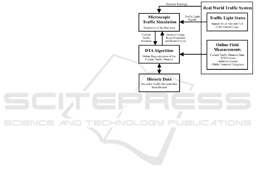
link past and future measurements. The structure of
the presented simulation-based method is sketched in
Figure 1. The block diagram shows how the real
world scenario interacts with the simulation and what
kind of data is used for which purpose. As mentioned
before, an essential aspect is the differentiation
between the online and offline processing and
calculations. There are several calculations which can
be performed prior to the actual simulation as a kind
of initialization process where for example average
travel times for each vehicle type combined with the
different traffic light states are computed. The
intervals of other state estimators are relatively large
(often minutes). The idea of adjusting a running
simulation and the outsourcing of calculations are
among others the reasons why very small update
intervals (a few seconds) can be used for this online
state estimation.
Figure 1: Block diagram of the presented DTA concept.
The main online field measurements in this
research consist of superior traffic counts, i.e. not
only a time stamp for crossing the detector, but also
the vehicle type and the current speed are detected via
radar technology. These detectors are so-called
TOPO-Boxes and this kind of detection is necessary,
because the future TLS control should contain a
vehicle specific prioritization. Nevertheless, the
concept is able to be enhanced by incorporating less
detailed measurements of induction loops and/or
PT telegrams (V2I communication type of specific
PT buses and the TLS). These additional sensor
information are inferior to those of the TOPO-Boxes
and therefore result in different interdependent levels
in the decision making process of individual vehicle
routing. The vehicle types within this whole approach
are generally classified according to the 8+1 class
defined by the German Federal Road Research
Institute (BASt) in (Bundesministerium für Verkehr,
Bau und Stadtentwicklung, 2012). Thus passenger
vehicles along with motorcycles, trucks, trailer etc.
are taken into account. Additionally bicycles are
detected so that the detection and the simulation are
extended to the so-called ‘8+1+F’ classification (RTB
GmbH & Co. KG, 2019).
VEHITS 2021 - 7th International Conference on Vehicle Technology and Intelligent Transport Systems
388

Subject to the variety of available data sources, the
algorithm has multiple routing levels. The most
important source allows the differentiation between
the above defined vehicle types. This is the reason
why the next subsection describes the highest routing
level in more detail (TOPO-Box Routing) and the last
subsection is dedicated to the interaction of all
considered and already mentioned levels.
3.2 TOPO-Box Routing
Since the TOPO-Boxes are mandatory due to their
type differentiation and their positioning between
successive TLS, this part of the paper dives deeper
into the mathematical description of the respective
dynamic problem. Some aspects of graph theory are
used to illustrate and explain the methodology of this
traffic estimation problem. Inspired by relevant
literature like (Bierlaire & Crittin, 2004), the traffic
network under research is modelled by a directed
graph to process the simulated data. The graph
is represented byits set of nodes and
its set of links . These nodes can either be
junctions or geometric points which meet the given
traffic infrastructure. The geometric points are the
discretization tool to model curves etc. which directly
influence the simulation, e.g. in terms of possible
speeds and accelerations. Streets of the complex
traffic system are therefore modelled through the
links . Special attention has to be paid to the
TLS-nodes
, as they play a central role in
controlling the system. In contrast to (Bierlaire
& Crittin, 2004), the sensors monitoring the system
are not directly represented by a subset of the links,
but as geometric points
. The graph does
only depend on the given infrastructure and not on the
time and is therefore used to describe the empty
traffic network. For all links the respective
travel time to reach each detector
is
calculated. For the presented approach it is important
that these travel times are stored prior to the actual
online simulation to determine the traffic state. Due
to different traffic light states and system loads, the
travel times will be modified over time. Any vehicle
state at any time can be accurately transmitted to the
data processing of the algorithm by the occupancy
vector
It contains the vehicle type, the current
speed and the current position on a specified edge of
each single vehicle such that
ℎ
vehicle type
ℎ
vehicle speed
ℎ
vehicle position
ℎ
vehicle's link
(1)
The time dependent traffic state can be represented
through this occupancy with
ℎ
being the
current number of vehicles in the system and each
vehicle type is associated with a different integer
(first entry of each row of
).
The aim of this theoretical construction is to help
assigning individual vehicles within the simulation to
specific sensors when there is a new measurement in
reality. The basic idea for the decision whether or not
a vehicle should be routed to a nearby sensor is to
check if the vehicle ‘fits’ to the corresponding sensor
measurement. The most important criteria to fit are
the accordance of measured and simulated vehicle
type and the needed travel time to reach the sensor.
Since the simulation has to run in real-time, the
simulation must be regularly adapted to the
measurements so that the traffic state can be well
estimated. Other criteria like the speed are less
appropriate, as they can be very discontinuous due to
curves, for example, and thus make the assignment
process more difficult. But since the speed is
measured, this information is used in a different way
to predict the future vehicle situation the best way
(explained later). It is a key aspect of the approach
that each of the mentioned vehicle types is handled
separately resulting in several subproblems.
Obviously there are several situations in complex
traffic systems where the route of vehicles has to be
assigned in different ways. In this DTA concept each
vehicle can be in any of the following positions to get
routed, which can be determined depending on the
current occupancy
and the current
measurements. The first case is that the respective
vehicles are not in reach of any sensor; i.e. the travel
time to arrive at any of the specified sensors lies
beyond a user-defined threshold of the algorithm.
This means that those vehicle cannot fulfill any of the
measurements. The second case is that vehicles are
close to just one sensor. Here it is determined that if
there exists a detection in the reality, the vehicle is
routed towards this sensor to satisfy the measurement
(i.e. ‘deterministic routes or vehicles’). The last
scenario is that vehicles are able to reach multiple
detectors due to their calculated travel time.
Depending on the measurements of these sensors it is
possible to construct an optimization problem which
minimizes the travel time and maximizes the
assignment of currently available vehicles
simultaneously (so-called ‘flexible routes or
vehicles’). The derivation of this binary optimization
problem follows.
The time discretization of the problem is
determined by the step size . Of particular
importance for the construction of the online
Online State Estimation for Microscopic Traffic Simulations using Multiple Data Sources
389

optimization problem is the difference between
deterministic and flexible routed vehicles. The
previous designation indicates that vehicles with just
one reachable detector can be directly assigned to the
respective detector, whereas the routes for vehicles in
a ‘flexible assignment area’ are not predefined. The
assignment of these vehicles to sensors that have
current demand is subject of optimization. The
complexity of this optimization problem depends on
the number of vehicles which are able to reach
multiple detectors as well as on the number of
reachable sensors
for each of these vehicles
. Because not all vehicles are even within
range of a single sensor it applies
. A flexible vehicle with its
reachable detectors results in
binary
optimization variables
which determine
whether or not a vehicle will be routed towards the
respective sensor. The total number of optimization
variables at the
th
step is
(2)
Because each of the vehicles can only be routed
once, the sum of all optimization variables for each of
the vehicles needs to be less than or equal to
. This leads to the first inequality conditions of the
optimization problem for the
th
time step
(3)
where
assigns the optimization variable
to the vehicle . In order to route
the exact number of detected vehicles in the
corresponding time interval to the respective sensors,
additional constraints are added to the problem
formulation. These constraints are based on the
number of sensors
and ensure that already
assigned deterministic vehicles are considered. This
second part of the restrictions yields to
(4)
with
assigning the optimization variable
to the sensor
being the total number of
measurements for sensor
being the number of already (in
this time interval) deterministically routed
vehicles to sensor
representing the measurements
still to be fulfilled for sensor
If there are more vehicles that can be
deterministically routed than measurements
(
), the adjusted field measurements
are set to zero, i.e.
and just the nearest
vehicles are routed.
Through this inequality constraints the
optimization problem can be formulated as
subject to
(5)
Just as already introduced, the objective
can be chosen to minimize the travel times of the
vehicles to satisfy the detections and simultaneously
maximize the number of assigned vehicles in the
simulation. In this case the objective would be
,
(6)
where
are the travel times for each vehicle
to the respective sensors,
describe weighting factors for travel
time and assignment
If the current demand of a specific sensor cannot
be satisfied through the assignment of available
vehicles, new vehicles have to be inserted into the
simulation to fulfill the measurement, i.e. the
inequality constraints in (4) are not met with equality.
Notice that these insertions or spawns lead to a
general consistency in terms of traffic counts and
their equivalents in reality are incoming vehicles from
unobserved side streets. Once a vehicle is assigned to
a detector in the simulation, it cannot be reassigned
until it reaches the desired detector. A follow-up
destination is set for each vehicle assignment, i.e. a
route prediction based on probabilities derived from
historical data is performed. The details of this
stochastic process will not be further discussed here.
It closes the gap between the matching of a field
measurement and the intrusion of a vehicle into an
area for successive routing. Without the follow-up
VEHITS 2021 - 7th International Conference on Vehicle Technology and Intelligent Transport Systems
390

routes there would be no routable vehicles for the
TOPO-Box Routing and all vehicles would have to be
spawned or generated. The data processing of the
historical ‘offline’ route prediction is done prior to the
main simulation and updated frequently during the
simulation. In doing so, a daytime-specific route can
be assigned to the vehicles online. This route can be
considered as less prioritized than the online route
choice determined by the optimization. The routable
vehicles for each vehicle type within the simulation
can be derived from the current occupancy
with an additional query whether the previous
destination has already been reached. In the end of
every simulation step there has to be a check if still
routable vehicles are about to cross a detector. Since
these vehicles were not assigned through the routing,
a crossing is not justified and the vehicles need to be
removed from the simulation to ensure the
measurements of reality. In reality, these vehicles
have entered unobserved roads or parking lots.
3.3 Interaction of Different Routings
The previous section points out the concept of the top
level routing, but there are two more implemented
levels which optionally help the traffic state
estimation to be more accurate. It is clear that the
more information and data the algorithm is capable of
processing, the more precise the traffic estimation can
become and the better the TLS-control can adapt to
the current traffic. The second routing level affecting
all types of vehicles is based on the induction loop
data. As they are widely used nowadays, this
information can complement the TOPO-Box
measurements without the need to buy additional
measuring equipment. For the purpose of controlling
TLS they are extremely worthy since the radar
technology is quite vulnerable in congested areas.
Therefore, the TOPO-Boxes are not set up in the
direct vicinity of an intersection. On the contrary, the
induction loops are usually only to be found in these
areas which is why the combination of data sources
can be particularly profitable. The third and last data
source uses V2I-technology, but exclusively for
regularly driving PT buses. Those buses transmit
their PT line number at specified locations within the
system when approaching and leaving TLS. Right
now it is already used to prioritize the PT, but in a
way that has a strong negative impact on the other
traffic and thus additionally leads to unnecessary
congestion.
Because of that, the TOPO-Box Routing is
extended in this approach with the so-called
Induction-Loop Routing and the PT-
Telegram Routing. The TOPO-Boxes are the most
detailed and reliable data source in terms of detecting
vehicles, but due to the relatively poor network
coverage and the network complexity it is still hard to
estimate the traffic state between measuring points.
The induction loops are lane based, so better capable
of detecting turning ratios at intersections and the
PT telegrams directly offer the future route of the
concerning bus since it is static. Figure 2 illustrates
the algorithm’s answer to the question how those
advantages can be combined. It shows the mutual
interaction (if allowed) of the different routing
concepts according to the drawn arrows. All routing
concepts have their own general spawn and routing
strategies, which change based on the vehicles’
previous assignments of other concepts.
Figure 2: Methods and interaction of the different routing
concepts.
To understand these interactions, it is important to
recall the principle of the TOPO-Box Routing. Here,
the vehicles (of all different types) get fixed routes
until passing the detector. Afterwards they are
equipped with flexible follow-up routes based on
stochastic turning ratios, historical data, etc. This
means that after crossing the aim detector an
‘educated guess’ is made how the vehicle will behave
until a successive measurement that fits the vehicle
comes up. As a consequence the routes of the non-
assigned vehicles (not assigned to a consecutive
TOPO-Box) can be manipulated to fit all different
data sources e.g. those of the induction loops. In
Figure 2 the boxes are divided into ‘spawn’ and
‘routing’. This addresses exactly whether a
corresponding vehicle in the vicinity of the sensor is
available for this routing or not. The routing level
interactions describe the vehicle handling depending
on the previously used routing. An arrow from the
Online State Estimation for Microscopic Traffic Simulations using Multiple Data Sources
391

Induction-Loop Routing to the TOPO-Box Routing
therefore implies the influence of the Induction-Loop
Routing on vehicles which have already been
assigned by the TOPO-Box Routing. As an example,
if a truck is detected by a TOPO-Box with no truck in
the vicinity of this sensor, a new one is spawned,
routed to this sensor and provided with a stochastic
follow-up route. Continuing this example, the truck
enters an intersection after crossing the TOPO-Box
with the desire to drive straight (derived from the
stochastic follow-up route). Suppose an induction
loop on the left turning lane is activated, then, as
indicated in Figure 2, the position of the truck is
changed and shifted to the left lane. Also, the route is
manipulated in such a way that the vehicle turns left
and approaches a destination in that direction.
Otherwise, if the target TOPO-Box location is behind
crossing the intersection straight, then the truck could
not be used for the Induction-Loop Routing. This is
because the left lane is not on the truck’s route, so the
change of position towards the induction loop
indicated by the arrow cannot be applied. Depending
on the absence of other vehicles a new one (passenger
type) would have to be spawned to match the
measurement. The usage of the PT telegrams is rather
simple and therefore kept short, since for buses the
educated guess can be swapped with the determined
fixed routes known due to the PT lines information.
After overwriting, the routes are fixed and the PT
buses can only be delayed or repositioned.
4 ALGORITHMIC PROCEDURE
For the traceability of the algorithm a step-by-step
guideline is presented in order to outline the
interaction of the microscopic traffic simulation
performed in SUMO (Lopez et al., 2018) and the
algorithmic data processing in MATLAB. First the
required traffic network for the simulation and the
correct representation of the traffic infrastructure has
to be built accurately in SUMO. This is a time-
consuming process, but clear due to the
unambiguousness of the infrastructure. The necessary
communication of microscopic traffic simulation and
data processing is realized with the interface
TraCI4Matlab (Acosta, Espinosa, & Espinosa,
2015).A brief summary of the concept to reproduce
the dynamics of the traffic system is as follows:
Step 0. Pre-Simulation calculation of all necessary travel
times. Loading and processing of historical data to
assign prediction routes (follow-up routes).
Initialization of the SUMO simulation.
Step 1. Change of the traffic lights according to the
recorded data and adaptation of the travel times.
Step 2. Check of the current vehicle situation in the traffic
system to decide their availability for the different
routing concepts.
Step 3. TOPO-Box Routing.
For each vehicle type: Solution of the integer linear
optimization problem.
a. Generation of the inequality constraints using the
current measurements and the simulation’s vehicle
states. Vehicles in areas with just one reachable
sensor within the travel time threshold are assigned
and given follow-up routes.
b. Performing of the integer linear optimization.
c. Assignment of the flexible vehicles resulting from
the optimization with determination of consecutive
destinations.
d. If there is still unsatisfied demand (leftover
detections), new vehicles of the respective type are
created and added to the simulation at the required
location with subsequent post-destination routes.
Step 4. Induction-Loop Routing.
Step 5. PT-Telegram Routing.
Step 6. Removal of vehicles that would cross the TOPO-
Boxes unwanted (no detection recorded at this time)
in the considered time interval.
If the desired simulation period is covered, stop,
otherwise return to step 1 for the next simulation step.
After this short overview some aspects will be
described in more detail. Prior to the initialization
step 0 the traffic network must be provided. Since
SUMO is used as simulation tool, its own network
editor NETEDIT (Lopez et al., 2018) is employed to
prepare the test area usually using OSM-data like in
(Feldkamp & Strassburger, 2014), but with the
SUMO-internal program OSMWebWizard. Also the
local sensors can be positioned here. To initialize the
simulation, the net information is employed to create
look-up tables including the travel times via
TraCI4Matlab. These tables store the travel times
depending on traffic light signals and vehicle types.
Since the road permissions for vehicles within the
network vary with their types and the simulation also
uses different general driving parameters, this
calculation procedure has to be done for each of the
vehicle types. A not further discussed offline-
algorithm determines the probabilities for the
follow-up routesup routes after reaching a destination
in the third step and also for step 4 beginning from the
induction loop lane. This algorithm tries to link traffic
counts of different detectors based on measurements
of the past creating routing probabilities. Even if no
historical data is available, random follow-up routes
can be assigned.
VEHITS 2021 - 7th International Conference on Vehicle Technology and Intelligent Transport Systems
392
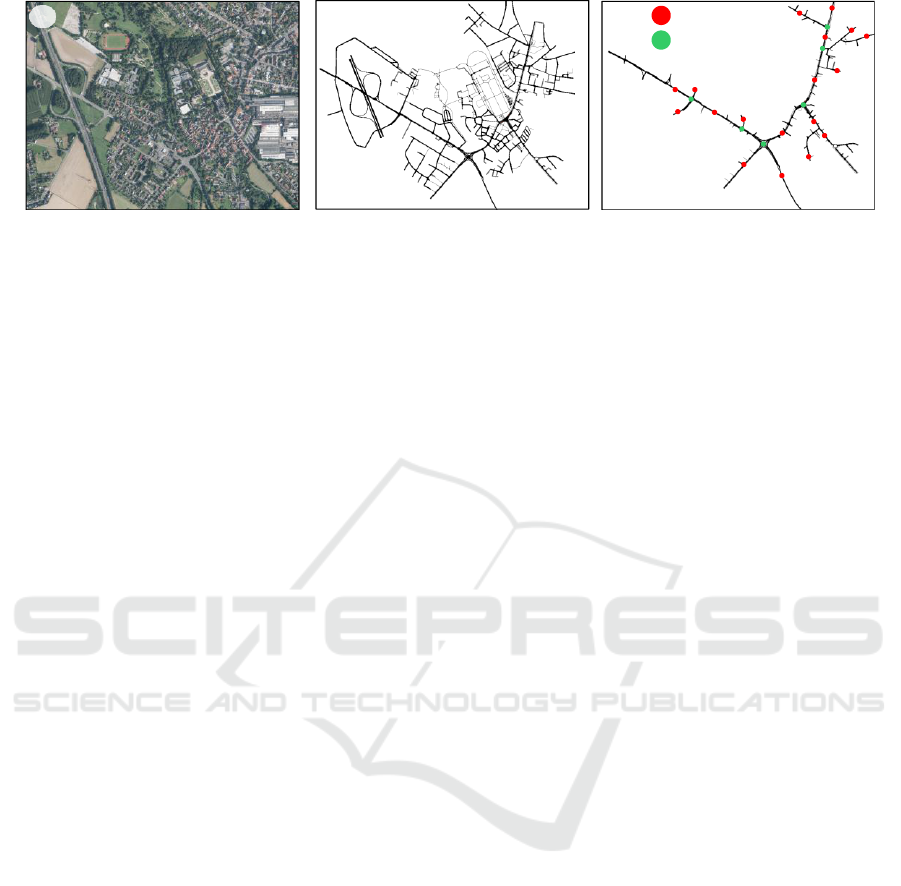
Figure 3: Transformation of the real test area in a) to the OSM-imported SUMO network in b) and its reduction to the
‘observable’ main roads equipped with the positions of TOPO-boxes and TLS in c).
After this preparation, the SUMO simulation can be
started. SUMO is used to handle the driver specific
behavior and mutual interaction between all vehicles
of all types. Each simulation step begins with the
setting of the current TLS signals and the query of the
current vehicle state. Based on an implemented
trigger, the routable vehicles with no fixed route are
filtered (follow-up routes from previous steps). The
filtering is followed by the different routing concepts
ordered according to their priority and ability to
interact with steps 3 to 5. Step 3 guarantees the
satisfaction of the detected vehicle demand through
whether deterministic, optimization based or
necessary leftover routing. These routing types are
superior to the follow-up routing after crossing a
detector. The superiority itself is realized by
overwriting the previous route. Since the TOPO-Box
measurements also include the vehicles’ speeds, the
velocity parameters of the routed vehicles are
adjusted through a simple not further explained
algorithm. For the removal of vehicles that do not
correspond to a field measurement, the routing trigger
and the distance to the upcoming detector is checked.
If a certain distance is underrun, the vehicle is
removed (step 6). As mentioned before, this
corresponds to unobservable events such as stopping
at parking lots or turning into unobserved roads or a
false route prediction. The procedure for the
reconstruction of the traffic state is highly sequential
which is why certain modifications can have positive
impacts in terms of efficiency. The removal of
vehicles has to be performed every simulation step for
each vehicle type whereas the vehicle assignment
based on the real-time data can be split for the types
and distributed on several seconds to increase the
efficiency without losing the consistency with field
measurements.
5 CASE STUDY
5.1 Test Area Setup
The chosen test area of the pilot project in Schloß
Neuhaus (Paderborn, Germany) covers a total area of
approximately
with multiple entries and exits.
In the following Figure 3 a bird's eye view of the real
road network in a) (Land NRW, 2019) is transferred
via the import of OSM data (OpenStreetMap
contributors, 2019) into a SUMO traffic simulation
network in b). Besides some necessary manual
adjustments, especially to replicate the real TLS and
the multimodality of the road permissions, the import
has been reduced by the unobservable roads (see c)).
The final network consists of a total of 441 nodes
(junctions and geometrical points) and 622 edges or
links including six TLS which will be object of future
optimization. These key numbers of the respective
graph are a result of a post-import discretization to
determine the travel times depending on the edges
more correctly because their length is limited to a
maximum of This way, a more time-
consuming online calculation can be avoided. The
real test area is equipped with around
20 TOPO-Boxes, which are also shown in Figure
3 c). Those detectors are capable of measuring the
current traffic for both directions of the road on which
they are installed. For this reason, twice the number
of sensors are inserted in the simulation at the
corresponding positions. Concerning the other data
sources, there are nearly 70 induction loops
surrounding the six TLS controlled intersections and
60 notification marks of the pt telegrams. The TLS
junctions are also illustrated in Figure 3 c). This
system architecture enables the application of the
routing without further adjustments.
TOPO-boxes
TLS
b) c)a)
Online State Estimation for Microscopic Traffic Simulations using Multiple Data Sources
393
5.2 Simulation Results
The approach was tested using several data sets from
different days in the near past, i.e. selected days in
October and November 2020 building various
scenarios with different vehicle loads. For the
following average data shown in Table 1, each of the
scenarios included a 30-minute time slot.
Table 1: Average deviation between real-life and
simulation measurements.
Total TOPO-Box Crossings
Total Induction Loop Crossings
Vehicle Speeds
The exceeding of the induction loop counts is based
on the lower priority of those measurements. The
TOPO-Boxes are the most important and reliable data
sources and therefore the Induction-Loop Routing is
not able to change already assigned vehicle routes.
Since Induction-Loop Routing itself tries to meet its
unfulfilled measurements, the number of crossings is
increased by because the rights to manipulate
the vehicle routes are intentionally missing (see
Figure 2). The vehicle speeds vary minimally
dependent on the higher local occupancy of the
system. Some intentional safety mechanisms in
SUMO prevent the exact mapping of the set speeds to
make the overall simulation more realistic. With this
system setup, the average speed deviation of
corresponds to a difference of less than
. If the
induction loop measurements prove to be more
reliable in the future, the occurring deviations can
even be reduced by allowing more interactions
towards the top level routing (see Figure 2 again).
Generally it can be said that due to the design of the
approach the TOPO-Box measurements are almost
perfectly approximated. But in order to get a better
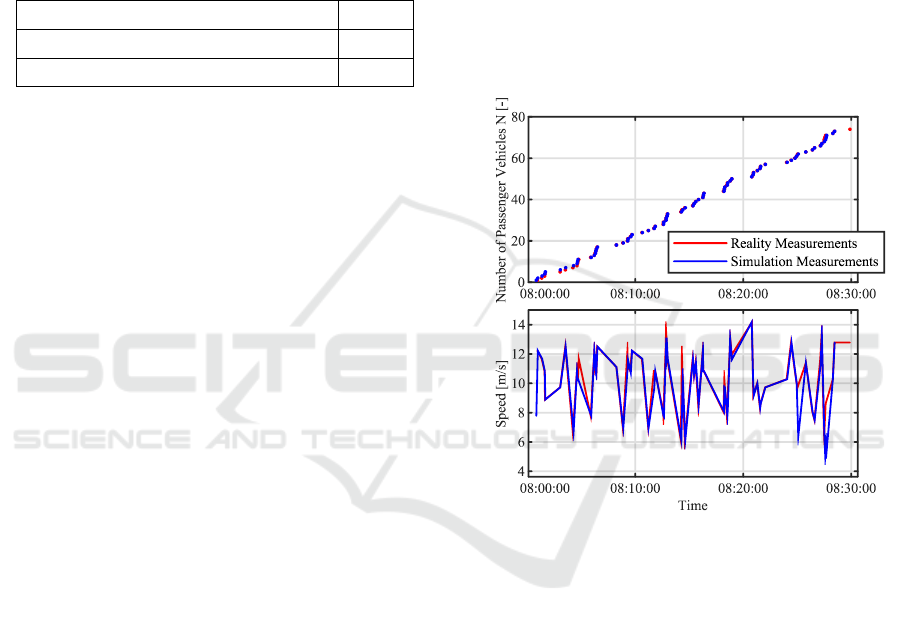
temporal breakdown of the results as well as some
explicit vehicle counts a specific example is given
below in Figure 4. It illustrates exemplary
measurements of the above mentioned time slots,
where each slot and each sensor provides comparable
results for each vehicle type. In the upper part of
Figure 4, the crossings of the passenger vehicles are
shown. The accordance of simulation and reality is
easy to notice as well as the absence of settling
processes. This is due to the fact that the time interval
used for all test results shown in this paper is only .
Additionally, the speeds for the corresponding
vehicles are pictured in the lower part of the figure.
The real average speed for this time slot is
and the simulated average is
.
The distribution of the induction loop crossings or
counts is not shown separately here, as it is
comparable to Figure 4 (with more deviation), but
does not include the same information because no
speeds are measured in reality. Due to the
PT-Telegram Routing there is nearly no deviation of
TOPO-Box crossings for buses ( ) since the
routes are fixed and the area coverage of the
telegrams together with the TOPO-Boxes allows
steady adjustments.
As a conclusion for the results, the estimation at
the local detection points (TOPO-Boxes and
induction loops) works very good and in combination
with SUMO also the speeds can be simulated
accurately.
Figure 4: Comparison of the reality and simulation
measurements for a single TOPO-Box regarding passenger
vehicles.
6 CURRENT & FUTURE WORK
The individual routes are not directly necessary for
the actual control of the traffic system. Since these
traffic records are also very expensive and difficult to
enforce in Germany, a simulated validation option is
preferred. This is why currently an extensive
validation study is performed using ground truth
models and surrogate data as suggested in (Antoniou
et al., 2014). First examples with some vehicle
convoys show good results, as the system states can
be estimated reliably, but the study still has to be
extended to a completely realistic traffic.
In the future, the presented method will have to be
improved while maintaining its generic character.
VEHITS 2021 - 7th International Conference on Vehicle Technology and Intelligent Transport Systems
394

Within possible enhancements it is important to take
note of an efficient implementation because of the
real-time capability. Also, topics like the robustness
to corrupted measurements have to be discussed more
detailed. At the moment incorrect detections are
compensated at the next sensor. In terms of sensor
coverage, at least the main roads of the network have
to be covered. Pedestrians are another aspect which
will be added to the simulation based on their
identification by pressing the corresponding push
buttons at the intersection. This information will be
taken directly from the TLS control unit.
In parallel, various TLS control concepts are
currently under development, which have to be
coupled with the presented traffic state estimator.
This coupling will become very interesting,
especially under the aspect of state estimations with
deviations from reality.
The last future issue addressed here is that to reach
the overall goal of controlling TLS in the field based
on such a state estimation, some additional interfaces
and latencies should be kept in mind. Especially their
common standards, i.e. in this project the OCIT
standard (OCIT Developer Group (ODG), 2019),
have to be considered.
ACKNOWLEDGEMENTS
The authors would like to thank all participants of the
Pilot Project Schlosskreuzung (PPS) for the provided
data. This paper is part of the PPS and funded by the
Ministry of Economy, Innovation, Digitalization and
Energy of North Rhine-Westphalia.
REFERENCE
Acosta, A. F., Espinosa, J. E., & Espinosa, J. (2015).
TraCI4Matlab: Enabling the Integration of the SUMO
Road Traffic Simulator and Matlab® Through a
Software Re-engineering Process. In M. Behrisch & M.
Weber (Eds.), Lecture Notes in Mobility. Modeling
Mobility with Open Data. 2nd SUMO Conference 2014
(pp. 155–170). Springer-Verlag.
Antoniou, C., Barcelo, J., Brackstone, M., Celikoglu, H. B.,
Ciuffo, B., Punzo, V., et al. (2014). Traffic simulation:
Case for guidelines. Luxembourg: Publications Office
of the European Union.
Antoniou, C., Ben-Akiva, M., & Koutsopoulos, H. N.
(2010). Kalman Filter Applications for Traffic
Management. In V. Kordic (Ed.), Kalman Filter. InTech.
Bierlaire, M., & Crittin, F. (2004). An Efficient Algorithm
for Real-Time Estimation and Prediction of Dynamic
OD Tables. Operations Research, 52(1), 116–127.
Bundesministerium für Verkehr, Bau und Stadtentwicklung
(2012). Technische Lieferbedingungen für Strecken-
stationen.
Chen, X., Osorio, C., & Santos, B. F. (2019). Simulation-
Based Travel Time Reliable Signal Control.
Transportation Science, 53(2), 523–544.
Feldkamp, N., & Strassburger, S. (2014). Automatic
generation of route networks for microscopic traffic
simulations. In A. Tolk (Ed.), 2014 Winter Simulation
Conf. (WSC 2014), 2848–2859, Piscataway, NJ: IEEE.
Kamal, M. A. S., Imura, J., Hayakawa, T., Ohata, A., &
Aihara, K. (2015). Traffic Signal Control of a Road
Network Using MILP in the MPC Framework.
International Journal of Intelligent Transportation
Systems Research, 13(2), 107–118.
Land NRW (2019). Karte Schloß Neuhaus. Datenlizenz
Deutschland -Namensnennung -Version 2.0 (www.gov
data.de/dl-de/by-2-0).
Lopez, P. A., Wiessner, E., Behrisch, M., Bieker-Walz, L.,
Erdmann, J., Flotterod, Y.-P., et al. (2018). Microscopic
Traffic Simulation using SUMO. In 2018 IEEE
Intelligent Transportation Systems Conference, 2575–
2582, Piscataway, NJ: IEEE.
OCIT Developer Group (ODG) (2019). Online Portal
Arbeitsgemeinschaft zur Standardisierung von
Schnittstellen in der Straßenverkehrstechnik.
OpenStreetMap contributors (2019). Schloß Neuhaus Map,
from https://www.openstreetmap.org.
Osorio, C. (2019a). Dynamic origin-destination matrix
calibration for large-scale network simulators.
Transportation Research Part C: Emerging
Technologies, 98, 186–206.
Osorio, C. (2019b). High-dimensional offline origin-
destination (OD) demand calibration for stochastic
traffic simulators of large-scale road networks.
Transportation Research Part B: Methodological, 124,
18–43.
Paz, A., Molano, V., Martinez, E., Gaviria, C., & Arteaga,
C. (2015). Calibration of traffic flow models using a
memetic algorithm. Transportation Research Part C:
Emerging Technologies, 55, 432–443.
RTB GmbH & Co. KG (Ed.) (2019). Produktprospekt
TOPO: Fahrzeug-klassifizierungssysteme. Deutsch-
land, Bad Lippspringe.
Wang, Y., Wang, D., Xu, B., & Wongpiromsarn, T. (2013).
Junction-based Model Predictive Control for urban
traffic light control. In 2013 International Conf. on
Connected Vehicles and Expo (ICCVE) (pp. 54–59).
IEEE.
Zheng, G., Zang, X., Xu, N., Wei, H., Yu, Z., Gayah, V., et
al. (2019). Diagnosing Reinforcement Learning for
Traffic Signal Control.
Online State Estimation for Microscopic Traffic Simulations using Multiple Data Sources
395
