
A Cooperative Platooning Controller for Connected Vehicles
Youssef Bichiou
1 a
, Hesham Rakha
1,2 b
and Hossam M. Abdelghaffar
1,3 c
1
Center for Sustainable Mobility, Virginia Tech Transportation Institute, Virginia Tech, Blacksburg, VA 24061, U.S.A.
2
Charles E. Via, Jr. Department of Civil and Environmental Engineering, Virginia Tech, Blacksburg, VA 24061, U.S.A.
3
Department of Computer Engineering and Systems, Engineering Faculty, Mansoura University, Mansoura 35516, Egypt
Keywords: Connected and Automated Vehicles, Platooning, Fleet Control.
Abstract: One of the key priorities of technologies is performance. In the area of transportation, performance is typically
intertwined with increased mobility and reduced costs. Congestion alleviation which is a persistent challenge
faced by many cities is a priority. The use of infrastructure is inherently inefficient, resulting in higher vehicle
fuel consumption and pollution. This in turn burdens commuters and businesses. Therefore, solving this issue
is of prime significance because of the potential benefit. Many technologies have been and are being
developed. These include adaptive traffic signals and various dynamic traffic control strategies. This paper
introduces a platooning controller that keeps relatively small time gaps between consecutive vehicles to
increase mobility, and eventually reduce travel costs. This controller also accounts for complex dynamic and
kinematic restrictions controlling vehicle motion. The controller is tested in a virtual environment on
highways in downtown Los Angeles. A drop-in travel time, delay, fuel consumption was observed across the
area for connected automated vehicles (CAVs) and non-connected vehicles, at various market penetration
rates (MPRs). Reductions of up to 5%, 9.4%, and 8.17% in travel time, delay, and fuel consumption,
respectively are observed. These observations are observed for all vehicles platooned and non-platooned.
1 INTRODUCTION
A dynamic phenomenon that requires sophisticated
modelling is roadway traffic. Nevertheless, different
properties can be observed directly. These properties
include (1) the density of the traffic stream (k): the
number of vehicles per unit length per road or lane;
and (2) the space-mean velocity (u): the density
weighted average velocity of the traffic stream.
Congestion is intertwined with high density and slow
space-mean speeds. Through designing technologies
that direct traffic and use the infrastructure as
efficiently as possible, researchers are attempting to
reduce traffic congestion. Wireless networking
advancements, ground breaking driver assistance
systems (Bevly et al., 2017) have made ideas
developed on paper become a reality. Platooning is
one of these ideas. Platooning is basically a group of
cars traveling at the same speed and keeping limited
space in between and is usually referred to as
a
https://orcid.org/0000-0002-0413-866X
b
https://orcid.org/0000-0002-5845-2929
c
https://orcid.org/0000-0003-4396-5913
cooperative adaptive cruise control (CACC). This
basic idea has the potential to boost transportation. Its
perceived benefits are efficient mobility, lower fuel
consumption, reduction in CO
2
emissions, and
increased highway capacity. Particular attention was
and is still being allocated to the development of
platoons. The work of Deng and Ma (Deng & Ma,
2014) utilized Pontryagin’s maximum principle
(PMP) to develop a platooning algorithm for trucks.
They claim up to 30% reduction in fuel consumption
on the deceleration regime and up to 3.5% in the
acceleration regime.
Al Alam et al. (Alam, Gattami, & Johansson,
2010) were inconclusive with respect to fuel
consumption reduction for platooned large vehicles
equipped with a commercial adaptive cruise control
(ACC). However, they reported a maximum energy
saving ranging from 4.7 to 7.7% with maximum
savings corresponding to a time gap of 1 s. They
acknowledged that a short time gap results in
maximum drag reduction, yet it comes with
378
Bichiou, Y., Rakha, H. and Abdelghaffar, H.
A Cooperative Platooning Controller for Connected Vehicles.
DOI: 10.5220/0010409003780385
In Proceedings of the 7th International Conference on Vehicle Technology and Intelligent Transport Systems (VEHITS 2021), pages 378-385
ISBN: 978-989-758-513-5
Copyright
c
2021 by SCITEPRESS – Science and Technology Publications, Lda. All rights reserved

challenges (i.e., feedback and communication delays)
which in turn threaten the safety as well as the
comfort of passengers.
Carl et al. (Bergenhem, Shladover, Coelingh,
Englund, and Tsugawa, 2012) reported various
platooning projects, namely, safe road trains for the
environment (SARTRE) (an European platooning
project), partial automation for truck platooning
(PATH) (a California traffic automation
program), grand cooperative driving challenge
(GCDC) (cooperative driving initiative), and
SCANIA platooning and energy ITS. They
emphasized the importance of connectivity V2X
which involves vehicle to vehicle (V2V) and vehicle
to infrastructure (V2I) communication, as well as
vehicular and non-vehicular sensors in allowing
platooning to address the issues of synchronization
and vehicle longitudinal and lateral stability.
Increased safety and reduced emissions were reported
by Davila et al. (Davila & Nombela, 2012) in the
SARTRE project. Virtual testing showed that better
engineered vehicle aerodynamics results in less
energy consumption. Platooning automation is
expected to enhance safety since 95% of accidents are
primarily caused by humans (Brown, 2005).
Other nationally funded projects targeting
platooning technologies were also unveiled. Within
the framework of the Japanese national intelligent
transportation system (ITS) project, Tsugawa et al.
(Tsugawa, Kato, & Aoki, 2011) created a system that
could assist vehicles to platoon automatically. They
showed that experiments on three fully autonomous
trucks operating at a speed of 80 km/h and a distance
gap of 10m (i.e., time gap of 0.45 s) results in 14%
fuel savings and hence a decrease in CO2 emissions.
In another study, a series of platooning tests on
large vehicles were performed. Michael et al.
(Lammert, Duran, Diez, Burton, & Nicholson, 2014)
tried different vehicle mass, speeds as well as distance
gaps in search for the optimum configuration
resulting in the highest energy consumption
reduction. This combination turned out to be a
cruising velocity of 88 km/h (55 mph) and a 9.1 m (30
ft) gap distance for a fuel saving of 6.4%. This
percentage is significant given the modest initial
investment. The unintended effects of platooning on
trucks, were highlighted by Ellis et al. (Ellis and
Gargoloff, 2015). They stressed the significant
aerodynamic drag reduction. However, if the gap-
distance is low (i.e., 5m), the air flow through the
engine is greatly decreased, resulting in the
continuous fan activation which in turn reduced
potential fuel economy. Different platooning
configurations for large vehicles on highways were
tested by Vegendla et al. (Vegendla, Sofu, Saha,
Kumar, & Hwang, 2015). Using computational fluid
dynamics, up to 23% reduction in fuel consumption
can be achieved by trucks traveling in a platoon. Yet,
two trucks traveling side by side on highways
consume 11% more.
Beside the technologies developed for heavy duty
vehicles similar technologies were and are being
developed for passenger cars. For instance, Stanger
and Del Re (Stanger and del Re, 2013) developed a
linear predictive control model that directly optimizes
the fuel consumption of the vehicles inside the
platoon. A simplified car-following model was
adopted, and a quadratic approximation of the fuel
consumption was chosen, they claim a 20% reduction
in fuel. Other elaborate models were also proposed.
For example, using a non-linear vehicle model,
Schmied et al. (Schmied et al, 2015) have developed
a non-linear model predictive control (NMPC) logic
that takes into account various non-linear constraints.
It is important to mention here that the nonlinear
nature of the model presents a computational burden
preventing its real-time implementation.
Nevertheless, the controller was tested using a
hardware-in-the-loop (HIL) configuration and the
authors claimed 13% reduction in fuel consumption
as well as 24% reduction in NO
x
emissions. With the
benefits provided by the platoon, it is important to
note some of the disadvantages it has. These
drawbacks are partly related to the extreme case.
Specifically, long platoons and platoons that are near
an entrance ramp do cause merging failures and
congestion, where the incoming vehicles find no
proper gap to merge (Wang, Maarseveen, Happee,
Tool, and Arem, 2019).
The present effort delivers a platooning logic
principally inspired by a change of variables. It
extends the literature in the following aspects: (1) it
considers platoons of arbitrary lengths; (2) the
platoons are formed and broken in a dynamic fashion;
(3) realistic vehicle dynamics are considered in the
plattoning and (4) the algorithm is tested on a large-
scale virtual implementation. In order to simplify the
analysis, and primarily due to the lack of an
aerodynamic drag coefficient function that
determines the subject force on the trailing vehicle
when the two considered vehicles are of significantly
different sizes (i.e., a truck and a car), this paper
addresses platoons composed only of passenger
vehicles. Buses and trucks are not considered. The
same algorithm will operate with all types of vehicles,
given that the correct dynamic behaviour information
associated with the considered vehicle is available. In
the following section, we detail the dynamic forces a
A Cooperative Platooning Controller for Connected Vehicles
379
vehicle can be subject to as well as the dynamic and
kinematic constraints. Details of the controller and
the simulation setup are presented in the same section.
In the third section, results are presented and finally
concluding remarks and future work are presented.
2 METHODOLOGY AND
FORMULATION
In this section, the vehicle dynamic model, associated
constraints, the proposed platooning controller as
well as the test settings are presented.
2.1 Vehicle Dynamic Model and
Constraints
Vehicles on the road are subject to various external
forces and constraints. These include, dynamic
forces, such as tractive and resistive forces, velocity,
and acceleration constraints (H. Rakha, Pasumarthy,
P., and Adjerid, S., 2009). The tractive force is
defined in Equation (1), the resistive force is the sum
of the aero dynamic resistance R
a
(Equation (2)),
rolling resistance R
r
(Equation (3)) and grade
resistance R
g
(Equation (4)). Therefore, the upper
bound for the acceleration is given by Equation (5)
(Hesham Rakha & Ahn, 2004; H. Rakha, Lucic,
Demarchi, Setti, & Aerde, 2001). The variables
introduced in Equations (1)-(7) are summarized in
Table 2.
(1)
(2)
(3)
(4)
(5)
The airflow subject to the current vehicle might
be altered due to the presence of another vehicle in
front. We introduce the drag corrective factor
to
capture the impact of platooning on the vehicle drag
coefficient (Equation (6)) (Hussein and Rakha, 2020).
(6)
where, is the gap in meters and , , and are
calibrated constants. The critical gap value,
depends on the type of the vehicle. Table 1 presents
the different parameters that can be used in the model
depending on the position of the vehicle in the platoon.
For further details about this model the reader is
referred to the work in (Hussein and Rakha, 2020).
Table 1: Values of the parameters for Equation (6), for
various vehicle positions in the platoon, based on (HUSSEIN
& RAKHA, 2020).
Vehicle
position
Parameters
Lead
-0.89
-1.67
1.02
-
Middle
-0.90
-0.51
1.14
39.62
Trail
0.60
0.12
1.14
79.75
The maximum deceleration a vehicle can experience
is given by Equation (7)
(7)
Table 2: Description of the various variables.
Variable
Description
driveline efficiency (unitless)
mass of the vehicle on the tractive axle (kg)
vehicle power (kW)
gravitational acceleration (m/s
2
)
coefficient of road adhesion or the coefficient of
friction (unitless)
air density at sea level (kg/m
3
)
vehicle drag coefficient (unitless)
altitude correction factor (unitless)
Drag a correction factor (unitless)
vehicle frontal area (m
2
)
rolling resistance constant that varies as a function
of the pavement type and condition (unitless)
second rolling resistance constant (h/km)
third rolling resistance constant (unitless)
total vehicle mass (kg)
roadway grade (unitless)
braking efficiency
where
and
are the absolute bounds for the
acceleration of the vehicle. However, when there are
other vehicles on the road collision avoidance is of
utmost importance. Therefore, another constraint on
the acceleration is introduced. This constraint has the
exclusive role of decelerating the vehicle to a velocity
that of the vehicle ahead of it while at the same time
keeping adequate spacing. To avoid collision, the
minimum deceleration is given by Equation (8).
(8)
where,
is the desired deceleration level,
(9)
VEHITS 2021 - 7th International Conference on Vehicle Technology and Intelligent Transport Systems
380

where,
is the velocity of the current vehicle,
is the velocity of the vehicle ahead of it,
is the
position of the current vehicle,
is the position of
the vehicle ahead, and
is the spacing at jam
conditions.
is the deceleration level
needed for the following vehicle to reduce its speed
to that of the vehicle in front with the stopping
distance being equal to the distance gap separating
them. Therefore, the acceleration of any given vehicle
needs to satisfy the following conditions.
(10)
The RPA car-following model (Hesham Rakha,
Pasumarthy, & Adjerid, 2009) accounts for the
constraints on the acceleration in the perspective of
velocity. The velocity of the vehicle following
another one needs to satisfy the condition presented
in Equation (11), (Bichiou & Rakha, 2019).
(11)
where,
,
,
,
,
is the free flow velocity,
is the velocity at
capacity (
based on empirical
observations),
is the jam density, and
is the
saturation flow rate. The car following model
presented in Equation (11) is enforced at all times
throughout the simulation.
2.2 Proposed Controller
In order to sustain a constant time gap between two
consecutive vehicles, the introduction of a controller
is necessary. The controller’s objective is to maintain
a constant/desired time gap (
(Loulizi,
Bichiou, & Rakha, 2019). This can be achieved by
driving the error function –which transforms the
desired time gap to a distance gap between two
consecutive vehicles– defined in Equation (12) to
zero. This can be accomplished by allowing
consecutive and corrective acceleration or
deceleration inputs to following vehicle. One of the
simple ways of achieving this is presented in
Equation (13).
(12)
(13)
where is a strictly positive real number. The
solution to Equation(13) is given by
which guaranties that
converges to zero as
time increases, provided is strictly positive.
Substituting Equation (12) into(13) leads to
(14)
namely,
(15)
Equation (15) requires knowledge of the difference in
position between two consecutive vehicles as well as
their respective velocities, which can be achieved by
having sensors on the vehicles or through V2V
communication. The presented controller has one
hyper-parameter (). The amount of data that needs
to be transferred between the vehicles is minimum
(i.e., the velocity and the position of the vehicle
ahead). It is also possible to avoid this transfer of
information by measuring the position and velocity of
the vehicle ahead using radar. It is also important to
note that the computed value for the acceleration
need to satisfy conditions presented in
Equation (10).
2.3 Simulation Setup
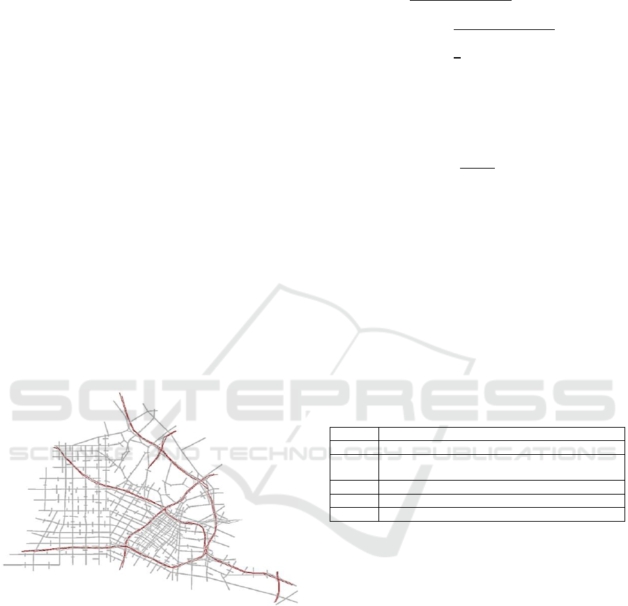
In this paper we consider testing the proposed
platooning controller on downtown Los Angeles,
specifically, the highway stretches that traverse it
from north to south and east to west. The total length
selected for the platooning is approximately 123 km.
The selected area is shown in Figure 1.
The network was modelled using the
INTEGRATION software (H. A. Rakha & Van
Aerde, 2020a, 2020b). The vehicle dynamic model,
dynamic constraints, and car-following model
presented in Section 2.1 are implemented in the
A Cooperative Platooning Controller for Connected Vehicles
381
software and are enforced all the time. The traffic
demand was calibrated using loop detector data by
computing the maximum likelihood static OD matrix
using procedures described in (Van Aerde, Rakha, &
Paramahamsan, 2003) and then adjusting the static
OD matrix to compute the dynamic OD matrix using
procedures described in (Yang and Rakha, 2019). A
detailed description of the calibration effort can be
found in (Du, Rakha, Elbery, and Klenk, 2018). This
resulted in a total of approximately 144,000 trips over
1-hour simulation. The selected highways do have
different lane counts. This count ranges from 3 lanes
to 6 lanes. For the purpose of this study, we selected
the two most left lanes as the lanes where we activate
platooning. In addition, we assumed a single vehicle
type, that is the 2018 Toyota Camry LE 2.5, one of
the most popular models sold in the USA. Its
characteristics are simulated in INTEGRATION
software. The fleet of Toyotas are subdivided into two
classes: class 1 and class 2. Class 1 are the Toyotas
that do not form or join a platoon (non-CACC
equipped vehicles). Class 2 are the Toyotas that do
form and if possible, join other created platoons
(CACC-equipped vehicles). The ratio of class 2 with
respect to class 1 was selected to be the variable to
discern the effects of various MPRs.
Figure 1: Downtown Los Angeles network, red represents
freeway links for platooning.
Vehicle’s fuel consumption is modelled using the
VT-CPFM-1 model presented in Equation (16) (Ahn
& Rakha, 2019), which is included in the
INTEGRATION software.
(16)
where, is the vehicle’s power and is the vehicle’s
velocity. The vehicle’s power is the product of the
force experienced by the vehicle and its velocity.
(17)
where,
(18)
and is the vehicle’s acceleration, this model was
validated in (Dion, Rakha, & Kang, 2004). The delay
that can be experienced by vehicles is computed using
Equation (19).
(19)
where
is the free flow velocity on a given link.
3 RESULTS AND DISCUSSION
In order to account for varying traffic conditions from
one day to another, simulations with various random
seeds were performed. First, we wanted to determine
the best platooning configuration to adopt. A series of
simulations were performed using the configurations
listed in Table 3.
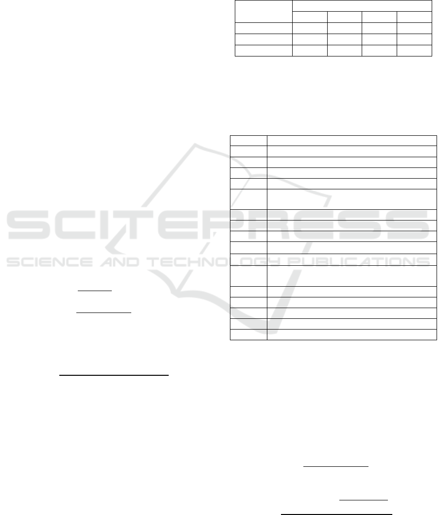
Table 3: Tested platooning configurations.
Config.
Details
A
Platooning on all lanes of the highway
B
Platooning on all lanes of the highway – platoon size
limited to 24 cars
C
Platooning on 1 lane
D
Platooning on 1 lane – platoon size limited to 24 cars
E
Platooning on 2 lanes – platoon size limited to 24 cars
Noting that in some configurations of Table 2 (B,
D, and E) platooning is enforced on individual links
in a disconnected manner from the links that follow.
The average link length is 500 m, the speed limit (i.e.,
platooning speed) is 25 m/s, the selected time gap is
(Loulizi et al., 2019), and a single
vehicle occupies 21 m. Therefore, 500 m contains
approximately 24 vehicles. Platoons are formed in a
dynamic manner. Any vehicle attempting to join a
platoon can increase its velocity by up to 7% beyond
the speed limit (i.e., platooning speed) for a maximum
duration of 6.5 s. If the vehicle is unable to join the
platoon within this time frame, a new platoon is
formed with this vehicle as a lead vehicle. These
parameters are user-specified and thus can be varied.
The average results of five random seeds are
presented in Table 4. It is clear from Table 4 that
configuration E has the best performance. This
VEHITS 2021 - 7th International Conference on Vehicle Technology and Intelligent Transport Systems
382
corresponds to travel time, delay and fuel
consumption reduction of 7.74%, 13.6% and 11.42%
respectively. This configuration stipulates that
platooning is enforced on the two leftmost lanes while
limiting the size of the platoon. Therefore, in the
subsequent simulations, we will only consider
configuration E.
Table 4: Results for the configurations in Table 3.
Travel
Time (s)
Total
Delay(s)
Fuel (l)
TT
Change
(%)
Delay
Change
(%)
Fuel
Change
(%)
Base
1032.6
561.7
0.89
A
1056.0
566.2
0.74
2.27
0.80
-16.48
B
1085.7
587.2
0.84
5.15
4.54
-5.50
C
993.3
513.4
0.88
-3.81
-8.60
-1.19
D
1036.6
568.0
0.88
0.38
1.13
-0.72
E
952.6
485.3
0.79
-7.74
-13.60
-11.42
In order to further investigate the effectiveness of the
platooning controller, we ran simulations with ten
random seeds at different MPRs. An average of the
results is presented in Table 5.
Table 5: Average performance metrics.
MPR
(%)
Travel
Time (s)
Total
Delay
(s)
Fuel (l)
TT
Change
(%)
Delay
Change
(%)
Fuel
Change
(%)
0
986.2
519.5
0.862
1
1008
538.2
0.873
2.19
3.60
1.28
5
980
511.7
0.857
-0.67
-1.50
-0.59
10
990
524.8
0.863
0.36
1.02
0.17
15
1005
536.0
0.868
1.92
3.19
0.72
20
1001
530.6
0.863
1.50
2.14
0.18
30
948
481.7
0.831
-3.93
-7.27
-3.61
40
961
497.2
0.836
-2.52
-4.28
-3.02
50
979
513.9
0.840
-0.75
-1.07
-2.58
60
945
481.8
0.813
-4.21
-7.25
-5.63
70
954
488.8
0.811
-3.31
-5.91
-5.91
80
937
470.7
0.791
-5.02
-9.40
-8.17
90
968
497.9
0.801
-1.81
-4.16
-7.09
100
995
522.8
0.809
0.85
0.64
-6.15
Table 5 shows the average travel time, delay and
fuel consumed for all vehicles in the network at
various MPRs. We can clearly discern that up to an
MPR of 20 % no significant advantage is provided by
the CACC platooning. In fact, the performance
metrics are about the same. Starting from an MPR of
30%, we observe a reduction up to 5% in travel time,
a reduction up to 9.4% in delay, and a reduction
between up to 8.17% in fuel consumption. It is
important to mention here that the RPA car-following
model and collision avoidance (Hesham Rakha et al.,
2009) are enforced at all times between all the
vehicles (platooned and non-platooned). This finding
demonstrates that efficient movement of a subset of
vehicles inside a large network leads to an improved
mobility for the entire network. Figure 2,
Figure 3, and Figure 4 present a scatter plot of the
reduction in travel time, delay and fuel consumption
reported in Table 5. Even though various seeds were
used for the simulation, the plots stress the reduction
in the mentioned performance metrics. The slope of
the decline of the fuel consumption is steeper than the
other measures of effectiveness. This is essentially
due to the significant reduction in the aerodynamic
Figure 2: Scatter Plot of the Travel Time Reduction
Percentage as a Function of the MPR.
Figure 3: Scatter plot of the delay reduction percentage as a
function of the MPR.
Figure 4: Scatter plot of the fuel consumption reduction
percentage as a function of the MPR.
y = -3,5268x + 0,3647
R² = 0,2319
-6,00
-4,00
-2,00
0,00
2,00
4,00
0% 20% 40% 60% 80% 100%
y = -6,7854x + 0,6521
R² = 0,2779
-12,00
-10,00
-8,00
-6,00
-4,00
-2,00
0,00
2,00
4,00
6,00
0% 20% 40% 60% 80% 100%
y = -8,9793x + 0,8381
R² = 0,8658
-10,00
-8,00
-6,00
-4,00
-2,00
0,00
2,00
0% 20% 40% 60% 80% 100%
A Cooperative Platooning Controller for Connected Vehicles
383

force to which the platooned vehicles are subjected
and therefore the vehicle needs less energy to
overcome that force. The slope for the reduction in
travel time, delay, and fuel consumption are
approximately -3.5%, -6.9%, and -9% respectively.
The respective coefficients of determination
are
0.23, 0.28, and 0.87 which further stresses the steep
reduction in fuel consumption due to platooning.
4 CONCLUSIONS
In this paper, an input minimal platooning controller
is presented. This logic takes into account various
dynamic and kinematic constraints that vehicles
experience. These include acceleration, velocity, and
collision avoidance constraints. This controller was
later applied on the highways in downtown Los
Angeles in the INTEGRATION software. The results
suggest a clear trend towards a reduction in system-
wide travel time, delay and notably fuel consumption.
The average reduction in travel time for all the MPRs
is up to 5%. The average reduction in delay as well as
fuel consumption (and ultimately CO
2
emissions) are
up to 9% and 8%, respectively. These results are for
the fleet of all vehicles, platooned and non-platooned
traveling through the downtown area. This leads us to
deduce that controlling the trips of a subset of
vehicles inside a large network does have the
potential to benefit other road users in a positive
manner. In the future work, we will be conducting a
detailed investigation on the performance of this
controller on a mixed platoon comprised of
conventional, hybrid and electrical vehicles at various
MPRs.
ACKNOWLEDGMENTS
This effort was funded through the Office of Energy
Efficiency and Renewable Energy (EERE), Vehicle
Technologies Office, Energy Efficient Mobility
Systems Program under award number DE-EE0
008209.
REFERENCES
Ahn, K., & Rakha, H. (2019). A Simple Hybrid Electric
Vehicle Fuel Consumption Model for Transportation
Applications. Retrieved from.
Alam, A. A., Gattami, A., & Johansson, K. H. (2010). An
Experimental Study on the Fuel Reduction Potential of
Heavy Duty Vehicle Platooning. Paper presented at the
13th International IEEE Conf. on Intelligent
Transportation Systems.
Bergenhem, C., Shladover, S., Coelingh, E., Englund, C.,
& Tsugawa, S. (2012, October 22-26). Overview of
platooning systems. Paper presented at the 19th ITS
World Congress, Vienna, Austria.
Bevly, D., Murray, C., Lim, A., Turochy, R., Sesek, R.,
Smith, S., Kahn, B. (2017). Heavy Truck Cooperative
Adaptive Cruise Control: Evaluation, Testing, and
Stakeholder Engagement for Near Term Deployment:
Phase Two Final Report. Retrieved from.
Bichiou, Y., & Rakha, H. A. (2019). Developing an
Optimal Intersection Control System for Automated
Connected Vehicles. IEEE Transactions on Intelligent
Transportation Systems, 20(5), 1908-1916.
Brown, I. D. (2005). Review of the 'looked But Failed to
See' Accident Causation Factor. Retrieved from.
Davila, A., & Nombela, M. (2012). Platooning - Safe and
Eco-Friendly Mobility. SAE International.
doi:10.4271/2012-01-0488.
Deng, Q., & Ma, X. (2014). A Fast Algorithm for Planning
Optimal Platoon Speeds on Highway. Paper presented
at the IFAC Proceedings.
Dion, F., Rakha, H., & Kang, Y.-S. (2004). Comparison of
delay estimates at under-saturated and over-saturated
pre-timed signalized intersections. Transportation
Research Part B-Methodological, 38(2), 99-122.
Du, J., Rakha, H. A., Elbery, A., & Klenk, M. (2018).
Microscopic Simulation and Calibration of a Large-
Scale Metropolitan Network: Issues and Proposed
Solutions. Paper presented at the Transportation
Research Board 97th Annual Meeting, Washington,
DC.
Ellis, M., & Gargoloff, J. I. (2015). Aerodynamic Drag and
Engine Cooling Effects on Class 8 Trucks in Platooning
Configurations. Paper presented at the SAE 2015
Commercial Vehicle Engineering Congress.
Hussein, A. A., & Rakha, H. A. (2020). Vehicle Platooning
Impact on Drag Coefficients and Energy/Fuel Saving
Implications. arXiv:2001.00560.
Lammert, M. P., Duran, A., Diez, J., Burton, K., &
Nicholson, A. (2014). Effect of Platooning on Fuel
Consumption of Class 8 Vehicles Over a Range of
Speeds, Following Distances, and Mass. Paper
presented at the SAE 2014 Commercial Vehicle
Engineering Congress.
Loulizi, A., Bichiou, Y., & Rakha, H. (2019). Steady-State
Car-Following Time Gaps: An Empirical Study Using
Naturalistic Driving Data. Journal of Advanced
Transportation, 2019. doi:10.1155/2019/7659496.
Rakha, H., & Ahn, K. (2004). Integration modeling
framework for estimating mobile source emissions.
Journal of transportation engineering, 130(2), 183-
193.
Rakha, H., Lucic, I., Demarchi, S., Setti, J., & Aerde, M.
(2001). Vehicle Dynamics Model for Predicting
Maximum Truck Acceleration Levels. Journal of
Transportation Engineering, 127(5), 418-425.
doi:10.1061/(ASCE)0733-947X(2001)127:5(418).
VEHITS 2021 - 7th International Conference on Vehicle Technology and Intelligent Transport Systems
384

Rakha, H., Pasumarthy, P., & Adjerid, S. (2009). A
simplified behavioral vehicle longitudinal motion
model. Transportation Letters: The International
Journal of Transportation Research, 1(2), 95-110.
Rakha, H., Pasumarthy, P., and Adjerid, S. . (2009). A
Simplified Behavioral Vehicle Longitudinal Motion
Model. Transportation Letters: The International
Journal of Transportation Research, Vol. 1(2), pp. 95-
110.
Rakha, H. A., & Van Aerde, M. (2020a). INTEGRATION
© Release 2.40 for Windows: User's Guide – Volume I:
Fundamental Model Features. Retrieved from
Blacksburg:
Rakha, H. A., & Van Aerde, M. (2020b). INTEGRATION
© Release 2.40 for Windows: User's Guide – Vol. II:
Advanced Model Features. Retrieved from Blacksburg:
Stanger, T., & del Re, L. (2013). A model predictive
cooperative adaptive cruise control approach. Paper
presented at the American Control Conf. (ACC), 2013.
Tsugawa, S., Kato, S., & Aoki, K. (2011). An automated
truck platoon for energy saving. Paper presented at the
2011 IEEE/RSJ International Conference on Intelligent
Robots and Systems.
Van Aerde, M., Rakha, H., & Paramahamsan, H. (2003).
Estimation of origin-destination matrices - Relationship
between practical and theoretical considerations. Travel
Demand and Land Use 2003(1831), 122-130.
Vegendla, P., Sofu, T., Saha, R., Kumar, M. M., & Hwang,
L.-K. (2015). Investigation of Aerodynamic Influence
on Truck Platooning. SAE International. doi:10.
4271/2015-01-2895.
Wang, M., Maarseveen, S. v., Happee, R., Tool, O., &
Arem, B. v. (2019). Benefits and Risks of Truck
Platooning on Freeway Operations Near Entrance
Ramp. Transportation Research Board, 2673(8).
Yang, H., & Rakha, H. A. (2019). A Novel Approach for
Estimation of Dynamic from Static Origin-Destination
Matrices. Transportation Letters: The International
Journal of Transportation Research, 11(4), 219-228.
doi:10.1080/19427867.2017.1336353.
A Cooperative Platooning Controller for Connected Vehicles
385
