Taxi Service Simulation: A Case Study in the City of Santa Maria

with Regard to Demand and Drivers Income

Andre Brizzi and Marcia Pasin

Programa de P

os-Graduac¸

ao em Ci

encia da Computac¸

ao, Universidade Federal de Santa Maria, Brazil

Keywords:

Simulation, Taxi Service, Drivers Income, Information System.

Abstract:

Taxi is an already well-established service in many cities around the world. Nowadays, the service request is

mainly made through mobile applications, where the user selects the desired options, including the payment

method. An information system, aware of the location of taxis, associates the closest taxi to the customer

request. In general, taxi allows the user to enjoy the mobility service without being directly charged by the

vehicle maintenance. The vehicle owner, who can be a company or a self-employed person (frequently the

taxi driver), is the one in charge with vehicle maintenance, fuel payment, etc. However, recently the taxi

service has lost much of its appeal due to competing car sharing services. Thus, it is necessary to evaluate

more carefully the implementation and maintenance of taxi service in cities with regard to the drivers income.

This work contributes in this way. Here, the taxi service is considered, with a standardized vehicle ﬂeet but

using different vehicle types (electric, ethanol, gasoline and CNG). Given a demand and costs, a simulation is

proposed to detail and evaluate the appropriate balance between drivers income and demand scheme to keep the

service viable to the drivers. Simulation was performed in a real scenario, the city of Santa Maria in Southern

Brazil. Input values in the simulation scenario (fuel price, demand, etc.) were chosen, based on literature,

city hall documentation and Internet news, to make the simulation as realistic as possible. Simulation results

shown that for feasible taxi service, the city town hall must deﬁne a maximum number of taxi licenses. The

vehicle type has a large impact in the taxi driver’s proﬁt. Electric vehicles have a lower cost per km driven,

but still have high cost of acquisition. Finally, if the daily traveled distance increases, the difference between

electric vehicles and the others decreases, making it possible electric vehicles to become more advantageous.

1 INTRODUCTION

Public transportation is known to be of poor quality in

many cities. And it is also known that there is a pref-

erence of passengers for individualized transportation

due to practicality, reliability, comfort, and safety. In

a recent survey (CNDL and SPC Brazil, 2017), 60.1%

of respondents who own private vehicles stated that

they would stop using it, if efﬁcient public transporta-

tion alternatives existed. In fact, the success of pro-

posals to improve urban mobility depends on mass ac-

ceptance by users (Alazzawi et al., 2018). The avail-

ability of tools and systems that bring together differ-

ent city mobility options is a key point for tracking

and understanding the city’s mobility needs.

One way to mitigate public transportation prob-

lems is vehicle sharing services, and one of the well-

established sharing services is the taxi. Nowadays, a

taxi service request is typically made through a mo-

bile application, where the costumer selects the de-

sired options, trip origin and destination, including

the payment method. In general, taxi allows the cos-

tumer to enjoy the mobility service without having to

pay the necessary amounts for the maintenance of the

car. An information system, aware of the location of

taxis, allows the taxi closest to the customer to meet

the request. The vehicle owner, who can be a com-

pany or a self-employed person (frequently the taxi

driver), is the one in charge with vehicle maintenance,

fuel payment, etc. However, recently the taxi service

has lost much of its appeal due to competing car shar-

ing services. Thus, it is necessary to evaluate more

carefully the implementation and maintenance of taxi

service in cities.

In this work, the taxi service is considered, with

a standardized vehicle ﬂeet. Given a ﬂeet size and

demand, a simulation is proposed to detail and evalu-

ate the pricing scheme with regard to the taxi demand

in a city. More speciﬁcally, we assess taxi drivers

income given a city demand and with regard to dif-

ferent vehicle types (electric, ethanol, gasoline and

CNG). Thus, questions we aim answer in this paper

Brizzi, A. and Pasin, M.

Taxi Service Simulation: A Case Study in the City of Santa Maria with Regard to Demand and Drivers Income.

DOI: 10.5220/0010406800310038

In Proceedings of the 23rd International Conference on Enterprise Information Systems (ICEIS 2021) - Volume 1, pages 31-38

ISBN: 978-989-758-509-8

include: How many runs does the driver have to make

per day/month to be worth it? Considering differ-

ent energy sources to the vehicle engines, what is the

source of energy most proﬁtable?

To run the simulation, we use SUMO (Behrisch

et al., 2011), a transportation network simulator with

open implementation. Simulation of the service is

performed in a real scenario, the city of Santa Maria

in Southern Brazil. In the simulation, we assume that

an information system manages the entire ﬂeet ser-

vice and associates customers with taxis, according

to a given demand. Input values in the simulation

scenario (ﬂeet size, demand, etc.) were chosen based

on literature, city hall documentation (Prefeitura de

Santa Maria, 2014) and Internet news, to make the

simulation as realistic as possible.

This paper is structured as following. Related

works are described in section 2. Simulation details

are described in section 3, and experiments in section

4. Conclusions are presented in section 5.

2 RELATED WORKS

In the literature, there are recent works that describe,

from the point of view of computer science and sim-

ulation, the behavior and the impact of shared vehi-

cles and taxis in transportation networks. The im-

pact of shared vehicles in the city of Milan, Italy,

was simulated with the aim of optimizing trafﬁc by

reducing the number of vehicles circulating in streets

(Alazzawi et al., 2018). The simulation combined au-

tonomous robot-taxis, with on-demand mobility ser-

vices. Data used in the simulation include the num-

ber of vehicles circulation on the streets and mobile

cellular network usage, to model the concentration

of passengers in some areas. The simulation takes

into account the following parameters: travel time,

travel speed, waiting time for passengers to board the

robot taxi, emission of pollutants and taxi conﬁgura-

tions (with different amounts of seats). An algorithm

matches robot-taxis and consumers. According to the

authors, to eliminate congestion in Milan, it would be

necessary to reduce by 30% the number of vehicles on

the roads. To reduce demand at peak times, a dynamic

pricing system, combined with other initiatives, could

be used to motivate users to travel other time periods.

According to the seats in each car, the more seats the

robot-taxi has, the longer the costumers will have to

wait and travel due to route deviations. Robot-taxis

with around 20 seats are indicated for long distance

travel. Robot-taxis with two seats allow better travel

ﬂexibility, but do not provide such a signiﬁcant reduc-

tion in city trafﬁc.

The combination of independent agent model sim-

ulators was also explored (Segui-Gasco et al., 2019).

MATSim (Horni et al., 2016) generates transportation

demand, associating costumers to mobility options

according to their preferences and IMSim

provides

an operational execution environment for transporta-

tion networks. By this combination, authors evaluated

the impact of mobility scenarios from different per-

spectives: costumers, service-operators and city hall.

The simulation was calibrated with data from London

trafﬁc control and MERGE Greenwich Consortium

(2017-2018). Evaluated metrics were optimum vehi-

cle ﬂeet size, vehicle type (traditional taxis and ride-

share vehicles), vehicle size (4 and 8 seating places),

vehicle occupancy, as well as wait and detour times

for each costumer. A main feature of the proposal

was the evaluation of the trade-off between quality of

service and demand. Thus, a service-operator may in-

vestigate how ﬂeet size and energy (or even the travel

duration) affect a pricing model.

Simulation was also carried out in order to com-

pare business models for vehicle rental services (Per-

boli et al., 2017). The comparative analysis highlights

aspects of different business models and solutions ap-

plied to improve service. Business models for vehi-

cle rental services can be vehicle delivery-receipt or

free-ﬂoating. In the delivery-receipt model, ﬂeet does

not need to be managed and relocated, but consumers

need to travel to a particular pick-up and release loca-

tion. In the free-ﬂoating model, vehicles can be re-

leased anywhere. The free-ﬂoating model tends to

better satisfy consumers, since there is no need to

travel to a particular pick-up location. However, it

requires ﬂeet management to guarantee the availabil-

ity of vehicles in some locations, i.e., the company

needs to take vehicles that are in points of less inter-

est to places of higher demand. In this scope, different

costumers proﬁles can be deﬁned: commuters (those

that travel from home to work), professional and ca-

sual. These proﬁles are randomly assigned to routes.

In addition, different vehicle types can be used, such

as electric and combustion vehicles. With regard to

the ﬂeet management, electric vehicles need more ef-

fort when compared to combustion vehicles, due to

recharging time and the need to ﬁnd a charging point.

Efﬁcient route optimization was proposed as an

opportunity to increase drivers revenues (Li et al.,

2017). A vacant taxi represents wasting of both fuel

and taxi driver time. Moreover, inefﬁcient routing

can create more trafﬁc in the city and consequently

more pollutant are emitted. Therefore, the Markov

Decision Processes can be used to maximize drivers

revenues by the application of an efﬁcient routing ap-

http://www.talon.world

ICEIS 2021 - 23rd International Conference on Enterprise Information Systems

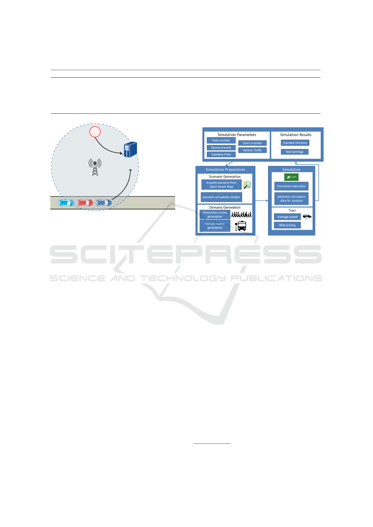
Table 1: Summary of related works.

Authors Vehicle type City Simulation platform

Alazzawi et al. 2018 Autonomous and Conventional Milan SUMO/TraCI

Segui-Gasco et al. 2019 Autonomous London MATSim/IMSim

Perboli et al. 2017 Conventional Turin none

Li et al. 2017 Conventional New York none

This work Conventional Santa Maria SUMO/TraCI

inf. system

costumer

Figure 1: An information system manages taxi ﬂeet and an-

swers client requests.

proach. Data from the taxi service from New York

City was used in the experiments. Simulation results

shown that the proposed model can collaborate to im-

prove drivers income since it reduces the time a cos-

tumer needs to ﬁnd a vacant taxi.

Related works are summarized in Tab. 1. Unlike

Alazzawi et al. and Segui-Gasco et al., which simu-

late the impact of using shared vehicles in cities, seek-

ing to reduce the number of vehicles in circulation

here, such as Perboli et al., we are focusing on the

provider side. In particular, in this work we are focus-

ing on the drivers income. Unlike Perboli et al. and

Li et al., and as in Alazzawi et al. and Segui-Gasco

et al., we use simulation to investigate how different

parameters impact the expected results and drivers in-

come.

3 PROPOSED SIMULATION

In this work, taxi service is considered in a simulation

to detail and evaluate the drivers income in the end of

journeys. Fig. 1 depicts the required Information Sys-

tem (IS) to support this service. Taxis publish their

locations in the IS (1) and customers make requests

(2). The IS allocates taxis according to the location of

the customers.

The simulation scheme, implemented in SUMO

trafﬁc simulator (Behrisch et al., 2011), is depicted in

Fig. 2 and consists of three main parts: scenario, input

Figure 2: Simulation scheme.

parameters and results. The scenario presents the map

of the geographic region to be simulated. The map has

tow layers: a static layer and a dynamic layer. The

static layer is previously obtained through a cut in the

map of Open Street Map

, exported in .osm format.

Using the SUMO Simulator script, the osm ﬁle

is converted into a transportation network, a scenario

formatted to be simulated by SUMO. The network is

composed by edges (street corners) and connections

between edges (street blocks). In the scenario conver-

sion, the path to the .osm ﬁle is indicated and addi-

tional parameters, such as the generation of sidewalks

along the roads can also be informed. After complet-

ing the stage of generating the map scenario, the out-

put is a ﬁle in .net.xml format (i.e., the description of

the transportation network). This map runs in a server

in which other simulation parameters can be conﬁg-

ured. For instance, the duration of the simulation.

The simulation parameters are sent to the simula-

tion server via Trafﬁc Control Interface (TraCI) (We-

gener et al., 2008). On the server side, the parameters

are used by the simulator generate the demand (i.e.,

the taxi runs) that associate costumers and taxis. Us-

ing the randoTrips.py script, provided by SUMO, ran-

dom trips are automatically generated, both for cos-

tumers and vehicles. We have the possibility to deﬁne

https://www.openstreetmap.org

Taxi Service Simulation: A Case Study in the City of Santa Maria with Regard to Demand and Drivers Income

parameters for this script such as:

• maximum distance that a costumers can walk,

• probability that a trip can start at the scene, and

• vehicle intensity ﬂow and costumers/pedestrians

ﬂow and, in addition, to establish which vehicle a

costumer can choose to complete her/his journey

trip.

The randoTrips.py script generates a ﬁle in the

.rou.xml format with valid routes to be used by

SUMO. The next step is running the simulation. The

SUMO simulations are presented by a .conﬁg ﬁle,

which contains the name of the ﬁle with the sce-

nario, .net.xml, of the additional items, .add.xml and

of the routes, .rou.xml. When loading the simulation,

SUMO searches for the information in the ﬁles pro-

vided. Also in the .conﬁg ﬁle, it is possible to deﬁne

the output to be presented after the simulation.

With regard to our simulation, some output in-

formation can be obtained automatically by SUMO

and include, for example, the vehicle average speed.

However, some speciﬁc routines have been coded,

since SUMO does not implement all the necessary

routines required in the scope of this work.

In general, simulation results that we are mainly

investigated in our scenario include:

• gross and net drivers incomes, with regard to the

number of runs, and

• drivers incomes, with regard to the vehicle type

(engine).

To summarize, the developed simulation receives

the data from the simulation ﬁles, and presents the

resulting values that we discuss in more details in the

section 4.

Parameters in our simulation deﬁned according to

real-world available data to drivers/taxis include:

• price of the fuel, vehicle model, etc.,

• monthly rental amount and vehicle consumption

related to the taxi model,

• formula to compute the payment for a taxi run,

which is composed by a ﬁxed amount and the

amount per km traveled,

• working hours for drivers, and

• number of available taxis.

Reference values are shown in Tab. 2. These val-

ues directly inﬂuence the driver’s revenue. Parameters

that can be deﬁned in the simulation, using city/trafﬁc

information, according to real-world observations in-

clude:

• intensity of the vehicles ﬂow in the scenario to be

deﬁned by counting the number of vehicles in a

given simulation interval,

• average travelled distance, deﬁned according to

the behavior of costumers in that region, and

• demand for runs, which can be calibrated using

information provided by city hall.

At the end of the simulation, the travel cost can

be computed and, therefore, the drivers income. The

travel cost depends on the period of the day and the

distance driven by the taxi driver.

4 EXPERIMENTS

In this section, we ﬁrst present the scenario setup tak-

ing into account the city of Santa Maria, then we de-

scribe the demand generation process, i.e., the addi-

tion of costumers in the simulation interested in rid-

ing a taxi. In the following, we describe the simula-

tion process, and ﬁnally, we focus on the simulation

results of our experiments.

4.1 Scenario Setup

In Santa Maria downtown, there are 14 taxi stops

which are part of our simulation map. We assume

that half of these points have 2 taxis and the other

half have 3 taxis, resulting in a total of 35 taxis in the

simulation. Fig. 3 presents a screenshot of our simu-

lation environment in SUMO, with a set of streets in

the center of Santa Maria city.

In general, the city has a very irregular layout in

its streets. Each red diamond in the green map rep-

resents a taxi station. Each blue square represents a

pick up or an unboarding point, manually chosen for

this simulation.

4.2 Demand Generation

The pedestrian (costumer) demand in our simulation

is generated by PersonFlows routine from SUMO, in

which people are inserted at different points on the

map. This component periodically generates pedes-

trians in a deﬁned location. Pedestrians follow a pre-

deﬁned route to reach their destination, being able to

get around on foot or using a taxi vehicle. Other vehi-

cles are not inserted in the simulation, but the effect on

the trafﬁc behaviour of the other vehicles (bus, trucks

and private vehicles) is due to the conﬁgured speed

limitation that the taxi can develop in the city.

The simulation in SUMO takes place so that the

vehicles present in a routing list are inserted in the

ICEIS 2021 - 23rd International Conference on Enterprise Information Systems

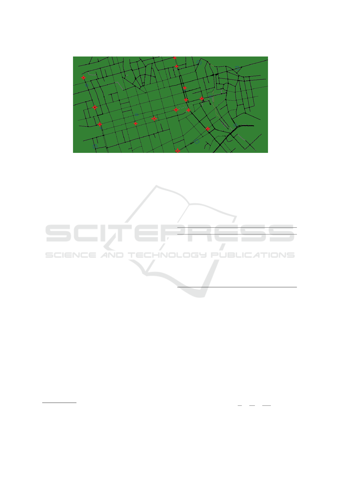
Figure 3: Screenshot of SUMO simulation environment.

simulation at the given time and after completing the

route these vehicles are removed from the simulation.

In order to make it possible for a taxi to perform mul-

tiple trips during the simulation, it is necessary to use

an auxiliary script to generate new routes for this ve-

hicle during the simulation. The script used for this

purpose is the Demand Keeper. This script is part of

the Net Populate

project, a set of scripts for gener-

ating and controlling demand in SUMO experiments.

Finally, Demand Keeper call is used in conjunction

with the TraCI interface, which allows to interact in

real time with SUMO.

4.3 Simulation Parameters and Drivers

Income

In the simulation, taxis are set to be in service from

8:00 a.m. to 4:00 p.m. Thus, we consider each taxi

service operates with three driver shifts per day, and

each taxi journey has the duration of 8 hours. Each

step of the simulation represents one second of time,

so the total number of steps in the simulation is 28,800

(i.e., 8 simulation hours). We run the simulation four

times, each time with an average demand for taxi rides

(i.e., 5, 10, 20 and 30 rides/day in average per taxi).

These values for the number of runs were chosen for

only 5 runs per day per driver to reﬂect a lockdown

scenario due to the new coronavirus pandemic, for in-

stance, and 30 runs would be a more optimistic sce-

nario. The number of costumers in each simulation

is modeled in order to create an average number of

rides per taxi in each simulation run. For simulation

purpose, we consider a standardized vehicle ﬂeet.

Simulation parameters are summarized in Tab. 2.

Each taxi run starts with an initial value called ﬂag

https://github.com/maslab-ufrgs/net-populate

, in which i = {0, 1, 2}, given the day of the week

and time, and the cost per kilometer traveled. The

values charged by the taxi drivers are stipulated by the

city hall (Araujo, 2020). Driver expenses also include

the fuel consumption per litre C, the maintenance cost

per kilometer traveled M, insurance expenses I, and

vehicle loan P.

Table 2: Simulation parameters.

Symb. Parameter Value

ﬂag-down fare 5.64 BRL/km

ﬂag-down fare 1 3.36 BRL/km

ﬂag-down fare 2 4.03 BRL/km

G fuel price 4.50 BRL/L

C fuel consumption tax 10 km/L

M vehicle maintenance 0.20 BRL/km

I annual insurance 2,000.00 BRL

P vehicle loan (monthly) 600.00 BRL

In addition to the parameters of Tab. 2, we add

that taxis move at an average speed of 36 km/h. For

the costumer-taxi association, we use the algorithm

implemented by SUMO where the taxi closest to the

costumer wins the run. In the simulation, we calculate

the gross income average obtained by taxis drivers

during the 8 hours of work, using Eq. 1 to compute

the individual Gross Income (GI) for each taxi driver:

GI = R · B

+ D

· B

, (1)

where R means taxi runs for the driver and D

means the total of the traveled distance (km). We also

compute the Net Income (NI) per taxi driver, using

Eq. 2, which is obtained by subtracting the vehicle

expenses from the gross amount, given by:

NI = GI − D

−

365

. (2)

Taxi Service Simulation: A Case Study in the City of Santa Maria with Regard to Demand and Drivers Income

100

150

200

250

300

350

5 10 20 30

Income (BRL)

Runs per working day

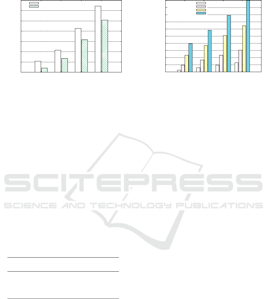
Figure 4: Values for GI and NI obtained in the experiment

using the parameters described in the Table 2.

We do not consider the amount paid in mainte-

nance of the vehicle in our equations, but this value

should be considered in a future study. In fact, some

values such as maintenance, insurance and ﬁnancing

can be shared by drivers who drive the same vehicle.

In the following, we highlight the simulation re-

sults of computing net and gross incoming and for taxi

drivers. We evaluate two different aspects: simulation

results with regard to drivers income and simulation

results with regard to the vehicle energy source.

4.4 Simulation Results with Regard to

Drivers Income

Here we assess the drivers income in different sce-

narios, from the pessimistic to the more optimistic.

Tab. 3 shows the simulation results for the average

travelled distance for costumers and drivers, given

different amounts of taxi runs.

Table 3: Travelled distance with regard to costumers and

total average distance, per driver.

Taxi Costumers Drivers total

runs (R) dist. avg. (km) dist. avg. (km)

5 7.7 12.6

10 14.9 21.5

20 29.8 45.5

30 45.2 65.8

In our simulation, the average distance traveled in

each trip is 1.5 km. In the most pessimistic scenario

(5 runs), the driver drives only 12.6 km per day, and

in the most optimistic scenario, the driver drives 65.8

km per day. Considering both scenarios (pessimistic

and optimistic), Fig. 4 depicts the (average) gross and

net values (GI and NI) obtained by the drivers per day

depending on the number of runs performed.

1000

2000

3000

4000

5000

6000

7000

8000

9000

10000

4 6 8 10

Income by month (BRL)

Working hours per day

5 daily runs

10 daily runs

20 daily runs

30 daily runs

Figure 5: Monthly NI based on working hours.

In Fig. 5, income values are plotted by month,

with regard to different number of working hours.

We, in particular, extrapolate the depicted values to

10 working hours. It is clear that the more the driver

works, the more she/he earns. However, if demand

is not enough, the driver is unable to pay the service

costs.

From the simulation results depicted in Figs. 4 and

5, we may conclude that it is impracticable to provide

taxi service in scenarios where the demand for taxi

runs is only 5 daily. Only 5 runs results in a monthly

gain of 952.24 BRL, less than the minimum wage cur-

rently in force by Brazilian legislation, given the law

number 14,013 (Brazil, 2020), which is 1045.00 BRL.

In contrast, if the taxi driver works in periods with de-

mands of 10 daily taxi runs, it is possible to guarantee

to the taxi driver an income above the minimum wage

working only 4 hours a day.

Given these results, it is important to highlight the

importance of balancing the amount of taxi licenses

allowed by the city hall and demand, in order to guar-

antee a sufﬁcient number of vehicles to serve passen-

gers while allowing the activity to remain proﬁtable

for taxi drivers. It is also important to observe that in

pessimistic scenarios, such as lockdown scenarios, for

instance, government contributions need to be consid-

ered for taxi service providers.

Another important observation is about the devi-

ation pattern we computed to the drivers income. In

our experiments, the deviation was quite high, as the

routing algorithm always ends up choosing the same

taxis that are closest to the passengers while other

taxis barely manage to run. For scenarios with high

demand, there is a greater turnover between taxis and

traveler origin points and destination points. There-

fore, a new algorithm to associate taxis and pedestri-

ans needs to be proposed in future work.

ICEIS 2021 - 23rd International Conference on Enterprise Information Systems

4.5 Simulation Results with Regard to

the Vehicle Energy Source

In addition to demand, another factor that impact the

taxi drivers income is the vehicle energy source. Here,

we consider three types of vehicles, according to the

energy sources:

• ﬂexible-fuel (ﬂex) vehicles, which are capable of

running with gasoline and ethanol,

• bi-fuel vehicles, which engines are capable of run-

ning on two fuels: a internal combustion engine

(with gasoline or diesel), and the other alternate

fuel such as natural gas (CNG), and

• electric vehicles, which are charged through the

electric power network.

In order to keep the vehicle in good condition, the

taxi driver changes her/his vehicle for a new one ev-

ery 5 years. Assuming that the taxi driver has a ﬂex

vehicle that is completing 5 years of use and needs

to change for a new one, she/he can choose from the

three types of vehicles mentioned above.

To purchase a new vehicle, we consider that the

driver current vehicle is worth 30,000.00 BRL, which

is used as an input for ﬁnancing. The ﬁnancing rate

is 1% monthly on average and the ﬁnancing term is

60 months. We emphasize that in Brazil, new vehi-

cles purchased by taxi drivers have tax incentives that

resulting in a value up to 30% less than paid by an or-

dinary consumer. We also considering that, in case of

CNG as energy source, typically, a conversion kit is

installed in the taxi and allows an originally ﬂex vehi-

cle to be supplied with CNG. The cost of installing a

CNG kit in a vehicle is 5,000.00 BRL on average.

To allow the evaluation of energy source, we con-

sider other values described in Tabs. 4 and 5. Tab. 4

shows the different types of vehicles and the respec-

tive installment to be paid. For ﬂex vehicles, the price

of the Renault Logan was considered, presented by

the manufacturer’s website in October 2020, for sale

with exemption for taxi drivers. The electric vehi-

cle chosen to the simulation was the one with the

lowest value found for sale currently in Brazil, JAC

iEV20. The price we used was according to the man-

ufacturer’s website in October 2020, considering an

exemption of 30% of the value for taxi drivers.

The choice of vehicle type in order to maxi-

mize driver proﬁt must take into account acquisition

cost and the cost per kilometre for travel. Tab. 5

presents vehicles comparison cost per travel kilome-

ter. Values for electric vehicle consumption we con-

sider here are based on the literature (Besselink et al.,

2011). Fuel price here used is based on the price

national survey carried out by the Brazilian National

100

150

200

250

300

350

5 10 20 30

Net income (BRL)

Rides per working day

electric engine

ethanol

gasoline

CNG

Figure 6: Drivers NI with regard to energy source.

Petroleum Agency

, relative to October 2020. In gen-

eral, ﬂexible-fuel vehicles have higher maintenance

costs when compared to electric vehicles (Alexander

and Davis, 2013). In contrast, electric vehicles have a

considerably high acquisition cost when compared to

vehicles with internal combustion engines.

Fig. 6 depicts our simulation results to drivers NI

based on energy source. Among the energy sources

we analyzed, it is possible to state that CNG max-

imizes the NI of taxi drivers in the scenarios of 20

and 30 daily taxi runs and ties with gasoline in the

scenario of 10 runs. For 5 daily runs, gasoline pro-

vides the highest proﬁt, with CNG being affected in

this scenario by the cost of installing the conversion

kit, which reﬂects in a higher installment value. Al-

though ethanol has a lower cost per liter than gasoline,

its autonomy has resulted in a lower NI than gasoline

in all scenarios.

Actually, the use of electric vehicles is not proﬁt

to taxi drivers when there are only 5 daily runs, but

as the number of daily runs increases, the difference

with regard to the proﬁt in relation to other energies

decreases. With 30 daily runs, the electric vehicle has

a proﬁt similar to a vehicle with ethanol. Although

it has the lowest cost per km traveled among all the

considered energies, the electric vehicle still has high

acquisition cost that results in large ﬁxed expenses,

harming the taxi driver’s NI.

5 CONCLUSIONS

This work proposed the evaluation of the taxi service

from the point of the view of the taxi driver (income).

The evaluation was conducted with simulation sup-

port, and considering an information system to deal

with entire taxi ﬂeet service and to associating cus-

tomers with taxis. From a real scenario, a simulation

http://preco.anp.gov.br

Taxi Service Simulation: A Case Study in the City of Santa Maria with Regard to Demand and Drivers Income

Table 4: Estimated vehicle acquisition cost.

Vehicle

type

First installment

(BRL)

Rate % a.m. Term

(months)

Final price (BRL) Installment

(BRL)

Electric 30,000.00 1 60 98,000.00 1,500.00

Flex 30,000.00 1 60 42,000.00 267.00

CNG 30,000.00 1 60 47,000.00 378.00

Table 5: Fuel comparison costs, given in kilometre per litre (Total) with regard to vehicle maintenance.

Vehicle type Price Mileage Maint. (BRL/km) Total (BRL/km)

Electric 0.50 (BRL/kWh) 0.2 (kWh/km) 0.10 0.20

Flex (ethanol) 4.00 (BRL/L) 7.0 (km/L) 0.20 0.77

Flex (gasoline) 4.50 (BRL/L) 10.0 (km/L) 0.20 0.65

CNG 3.72 (BRL/m

) 12.3 (km/m

) 0.20 0.50

from a service journey was performed.

Simulation results shown that for the taxi service

to be feasible for drivers, the city town hall must

deﬁne a maximum number of taxi licenses in order

to ensure that the average daily travel per driver is

not less than 10 runs. Smaller values mean that the

monthly taxi gain does not reach the minimum wage

established by the Brazilian government. The mini-

mum number of taxis allowed in a region must con-

sider the quality of the service, so as not to compro-

mise the availability of the service to costumers.

Vehicle type has a large impact in the taxi driver’s

proﬁt. Simulation results showed that although elec-

tric vehicles have a lower cost per km driven, the high

cost of acquisition made the taxi driver’s net proﬁt re-

sult in lower values than other types of vehicle. Fi-

nally, we mention that as the daily traveled distance

increases, the difference between electric vehicles and

the others decreases, making the new technology to

become more advantageous.

REFERENCES

Alazzawi, S., Hummel, M., Kordt, P., Sickenberger, T.,

Wieseotte, C., and Wohak, O. (2018). Simulating the

impact of shared, autonomous vehicles on urban mo-

bility - a case study of Milan. SUMO 2018- Simulat-

ing Autonomous and Intermodal Transport Systems -

EPiC Series in Engineering, 2:94–110.

Alexander, M. and Davis, M. (2013). Total cost of own-

ership model for current plug-in electric vehicles. In

TECHNICAL REPORT 3002001728. Electric Power

Research Institute (EPRI).

Araujo, M. (2020). Prefeitura de Santa Maria concede, ap

es anos sem aumento, reajustes nas tarifas de t

axis.

https://www.santamaria.rs.gov.br/noticias/20395-

prefeitura-de-santa-maria-concede-apos-tres-anos-

sem-aumento-reajustes-nas-tarifas-de-taxis.

Behrisch, M., Bieker, L., Erdmann, J., and Krajzewicz, D.

(2011). SUMO - simulation of urban mobility (an

overview). In Proc. 3rd Int. Conf. on Advances in Sys-

tem Simulation (SIMUL 2011), pages 63–68.

Besselink, I. J., Hereijgers, J., Van Oorschot, P., and Nijmei-

jer, H. (2011). Evaluation of 20000 km driven with a

battery electric vehicle. EEVC - European Electric

Vehicle Congress, Bruxelles, pages 1–10.

Brazil (2020). Lei n

14.013, de 10 de junho de 2020.

CNDL and SPC Brazil (2017). H

abitos e Prercepc¸

oes sobre

a Mobilidade Urbana no Dia a Dia dos Brasileiros.

SPC Brazil.

Horni, A., Nagel, K., and Axhausen, K. W. (2016). The

multi-agent transport simulation MATSim. Ubiquity

Press London.

Li, P., Bhulai, S., and van Essen, J. T. (2017). Optimization

of the revenue of the New York city taxi service using

markov decision processes. In Proc. 6th Int. Conf. on

Data Analytics, pages 47–52, Barcelona (Spain).

Perboli, G., Ferrero, F., Musso, S., and Vesco, A. (2017).

Business models and tariff simulation in car-sharing

services. Transportation Research Part A: Policy and

Practice, 115.

Prefeitura de Santa Maria (2014). Lei municipal n

5.863,

de 09 de maio de 2014.

Segui-Gasco, P., Ballis, H., Parisi, V., Kelsall, D. G., North,

R. J., and Busquets, D. (2019). Simulating a rich

ride-share mobility service using agent-based models.

Transportation 46, pages 2041–2062.

Wegener, A., Piorkowski, M., Raya, M., Hellbr

uck, H., Fis-

cher, S., and Hubaux, J.-P. (2008). TraCI: An interface

for coupling road trafﬁc and network simulators. 11th

Communications and Networking Simulation Sympo-

sium (CNS), pages 155–163.

ICEIS 2021 - 23rd International Conference on Enterprise Information Systems