
Condition Monitoring for Air Filters in HVAC Systems with Variable
Volume Flow
Oliver Gnepper
a
and Olaf Enge-Rosenblatt
b
Fraunhofer Institute for Integrated Circuits IIS, Division Engineering of Adaptive Systems EAS,
Zeunerstraße 38, 01069, Dresden, Germany
Keywords:
Condition Monitoring, Data Analytics, HVAC System, Air Filter, Smart Building.
Abstract:
State of the art condition monitoring systems for air filters in HVAC systems require that the HVAC system
is operated at nominal volume flow. For HVAC systems with variable volume flow this assumption is only
fulfilled in one operating point. Outside this operating point existing condition monitoring systems assess
the air filter condition in a too optimistic manner. Therefore, polluted air filters remain undetected until their
regular check, leading to unneeded energy consumption. If the true condition of an air filter is known, it could
be changed before it is clogged. So, a condition monitoring systems is needed which is also reliable in case of
HVAC systems with variable volume flow. This work presents a model-based approach for such a condition
monitoring system. Therefore, a dataset from a building is used to assess an optimal model. Furthermore, the
condition monitoring systems is evaluated on that dataset.
1 INTRODUCTION
Air filters in HVAC systems are used for precipitat-
ing of dust particles from the intake air. Addition-
ally, they protect succeeding components of an HVAC
system from pollution and damage due to abrasion.
Furthermore, particles which are harmful to human’s
respiratory system should be removed from the sup-
ply air as well. Therefore, it is necessary that air fil-
ters are in a good condition at any time. This is en-
sured by a professional service on a regular basis. In
(Verein Deutscher Ingenieure, 2018) a quarterly vi-
sual inspection is demanded and a semestral check of
the differential pressure of air filters in HVAC sys-
tems. For HVAC systems with a nominal volume flow
of more than 1000 m
3
/h, sensors which display the
current value of the differential pressure must be in-
stalled (Verein Deutscher Ingenieure, 2018). Usually
the measured differential pressure is compared with a
fixed limit to determine if an air filter is clogged and
must be changed. In principle, the differential pres-
sure measured at an air filter depends on the volume
flow which passes through the air filter. So, in case
of HVAC systems with variable volume flow a com-
parison of the differential pressure with a fixed limit
a
https://orcid.org/0000-0001-6430-620X
b
https://orcid.org/0000-0002-6069-7423
results in an erroneous estimation of the air filter con-
dition.
The following section contains a review of the
air filter condition monitoring state of the art. It is
shown that several approaches to monitor the air fil-
ter condition exist, but these approaches are either re-
stricted to be used in combination with a dedicated
HVAC system or high effort is necessary to retrofit
these approaches in existing HVAC systems. Further-
more, it is shown that several models of air filters exist
which could be used to estimate the air filter condi-
tion. These models are described in Section 3. For
each model the quality of fit is evaluated on a dataset
from a building in Germany. This dataset is described
in Section 4. The model selection method and the
corresponding results are shown in Section 5. In Sec-
tion 6 it is shown how the selected model is used to
monitor the condition of air filters. This work is fin-
ished with a conclusion in Section 7.
2 STATE OF THE ART
Detecting if air filters in HVAC systems with variable
volume flow are clogged, is a problem which is ad-
dressed in different ways. A pneumatic air filter con-
dition indicator for HVAC systems which displays the
air filter condition for two different fan speeds is de-
102
Gnepper, O. and Enge-Rosenblatt, O.
Condition Monitoring for Air Filters in HVAC Systems with Variable Volume Flow.
DOI: 10.5220/0010405401020109
In Proceedings of the 10th International Conference on Smart Cities and Green ICT Systems (SMARTGREENS 2021), pages 102-109
ISBN: 978-989-758-512-8
Copyright
c
2021 by SCITEPRESS – Science and Technology Publications, Lda. All rights reserved

scribed in (Ladusaw, 1966). The air filter condition
is indicated by a device which floats in the air that
bypasses an air filter. The floating height is also in-
fluenced by the fan speed. So, there is an indication
area for the low and the high fan speed. In (Fraden
and Rutstein, 2007) a method is described which uses
a heated wire to measure the volume flow. If the lat-
ter drops below a predefined limit, the air filter is de-
clared to be clogged. A similar method is claimed in
(Kang et al., 2006). Herein, the temperature gradi-
ent due to a fan speed change is measured. The air
filter condition is determined by comparing the tem-
perature gradient with a predefined limit. All these
approaches have in common that they detect air filter
clogging, but they are not able to predict the remain-
ing useful life of air filters. In addition to that these
methods must be tuned for different types of air fil-
ters.
An air filter model which utilizes measurements
that are already collected in HVAC system provides
a better scalability of the desired solution. In (Kang
et al., 2007) it is claimed that deviations of the to-
tal pressure difference of fans are mainly induced by
air filters. Therefore, the condition of an air filter is
assessed by comparing the measured total pressure
difference with the one which is estimated from the
characteristic fan curve. The total pressure difference
is truly affected by the condition of air filters, but this
is not the only influence. Therefore, this approach is a
good measure for anomalies in HVAC systems. This
method is designed for a particular system and does
not generalize well. Therefore, it is necessary to use a
model of air filters which represents the resistance of
air filters to the air flow.
In (Saarela et al., 2014) a model which combines
different influences on the differential pressure devel-
opment of air filters for nuclear power plants is intro-
duced. Each influence is modelled separately. Hereby
the relationship between volume flow
˙
V and differen-
tial pressure ∆p of an air filter is described by a model
of the form which is shown in Equation 1. This equa-
tion also includes the parameters a and n. Hereinafter
this model is called type I.
∆p = a ·
˙
V
n
(1)
In (Liu et al., 2003) such a model is also used to
estimate the reduction of empty spaces between fibres
of air filters. The same model structure is also de-
scribed in (DIN Deutsches Institut f
¨
ur Normung e.V.,
2013). Whereas, (Eckhardt, 2018) uses the following
approach to model the relationship between volume
flow and differential pressure of an air filter which is
subsequently denoted as type II.
∆p = a ·
˙
V
2
(2)
This modelling approach is also used in (Kruger,
2013) and in (Verein Deutscher Ingenieure, 2004).
The latter cites (L
¨
offler, 1988) which extends the sec-
ond order term with a linear term and the associated
parameter b. This yields Equation 3. The correspond-
ing model is consecutively called type III and is also
proposed in (Kanaoka and Hiragi, 1990), (Rivers and
Murphy, 2000) and (Albers, 2017).
∆p = a ·
˙
V
2
+ b ·
˙
V (3)
As shown, in the literature there is no standard
model for air filters. In addition, there is no com-
parison with other models in any of the publications.
Furthermore, there is no agreement in the literature on
the consideration of further influences on the differen-
tial pressure, such as air density or dynamic viscosity
of air as well as filter-specific parameters such as fi-
bre thickness. While the models in (Verein Deutscher
Ingenieure, 2004), (L
¨
offler, 1988), (Kanaoka and Hi-
ragi, 1990) and (Rivers and Murphy, 2000) cover
any of these influences in detail, the model in (DIN
Deutsches Institut f
¨
ur Normung e.V., 2013) takes only
the influences of air density and dynamic viscosity of
air into account. On the other hand the models in
(Saarela et al., 2014), (Liu et al., 2003), (Eckhardt,
2018), (Kruger, 2013) and (Albers, 2017) neglect all
influences. Therefore, for a comparison of these mod-
els, it is necessary to unify the level of detail of the
models and to adapt all models in such a way that it
is possible to quantify the benefit of further measured
variables and derived influences, such as air density
and dynamic viscosity of air.
3 FILTER MODELS
During the model unification, it must be ensured that
the resulting models can be retrofitted in existing
HVAC systems with as little effort as possible. In
existing HVAC systems, the filter-specific parameters
are usually unknown. Therefore, the level of detail
of the models is reduced to such an extent that they
do not contain any filter-specific parameters. Further-
more, it must be ensured that all used models can
represent the influences of air density and dynamic
viscosity of air. The following chapters describe the
model unification procedure and the resulting models.
3.1 Exponential Model
In (DIN Deutsches Institut f
¨
ur Normung e.V., 2013)
a model is described which takes dynamic viscosity
of air and air density into account and has the same
Condition Monitoring for Air Filters in HVAC Systems with Variable Volume Flow
103

structure as model type I. Equation 4 shows the cor-
responding mathematical statement.
∆p = c · µ
2−n
· ρ
n−1
·
˙
V
n
(4)
This equation includes a resistance coefficient c,
dynamic viscosity of air µ, air density ρ and an expo-
nent n. The latter is not restricted to a specific value
and changes over time as the dust load increases.
In (DIN Deutsches Institut f
¨
ur Normung e.V., 2013)
Equation 5 is used to calculate the dynamic viscosity
of air where T is measured in °C and µ in Pas.
µ =
1.455 · 10
−6
· (T + 273.15)
0.5
1 +
110.4
T + 273.15
(5)
The Equations 6 to 10 can be used to estimate
the air density which include the ambient pressure p,
the water vapour partial pressure p
w
and the relative
air humidity ϕ (DIN Deutsches Institut f
¨
ur Normung
e.V., 2013).
ρ =
0.378 · p · p
w
287.06 · (T + 273.15)
(6)
p
w
=
ϕ
100
· exp(c
1
−
c
2
T + 273.15
− c
3
· ln(T + 273.15))
(7)
c
1
= 59.484 085 (8)
c
2
= 6790.4985 (9)
c
3
= 5.028 02 (10)
The building in which the data is collected which
is used for the validation has two HVAC systems with
humidification and one HVAC system without hu-
midification (see Section 4). The ambient pressure
is measured in none of these HVAC systems. Addi-
tionally, the relative air humidity is only measured in
the two HVAC systems with humidification. In order
to include the influence of the air density, it is cal-
culated in two ways. In case of the HVAC systems
with humidification the Equations 6 to 10 are used,
but it is assumed that the ambient pressure is constant
at p = 101325Pa. Additionally, for all three HVAC
systems Equation 11 is used to estimate the air den-
sity (Albers, 2017). It is analysed which of the two
approaches provides more accurate results and thus
represents the preferred variant for similar cases (see
Section 5).
ρ = 1.275 ·
273.15
T + 273.15
(11)
3.2 Second Order Models
The model which is described in (Verein Deutscher
Ingenieure, 2004) bases on the model in (L
¨
offler,
1988) and is shown in Equation 12.
∆p =
2 · c
D
· u
2
· ρ · α · z
π · d
F
(12)
This equation includes the resistance coefficient
c
D
, the flow velocity u, the fibre layer thickness z,
the packing density α and the fibre diameter d
F
. The
last three parameters are constant. Only the pressure
coefficient, the differential pressure ∆p, the air den-
sity ρ and the flow velocity vary over time. The flow
velocity is not measured in the analysed dataset (see
Section 4), but is replaceable by the following expres-
sion which introduces the volume flow
˙
V and the filter
area A. The latter decreases over time as the dust load
increases.
u =
˙
V
A
(13)
As described above, Equation 13 is inserted in
Equation 12 which yields Equation 14. The filter-
specific parameters and the pressure coefficient are
substituted by the parameter c.
∆p = c ·
˙
V
2
· ρ (14)
In (L
¨
offler, 1988) this model is extended by an ad-
ditional linear term. This yields Equation 15. The
parameters c
4
and c
5
in Equation 15 replace the filter-
specific constants and any immeasurable coefficient
(e.g. filter area) which correspond to the dust load of
an air filter.
∆p = c
4
· µ ·
˙
V + c
5
· ρ ·
˙
V
2
(15)
The models in Equation 4, 14 and 15 have in com-
mon, that they describe the relationship between dif-
ferential pressure and volume flow of an air filter, but
they differ in their structure. All three models take the
influence of the air condition (dynamic viscosity and
density) into account. The dynamic viscosity of air
is calculated as described in Equation 5. In the case
of air density, it depends on whether the relative air
humidity is measured. If this is the case, then Equa-
tions 6 to 10 are applied. If this is not the case, then
Equation 11 is used. The different models in combi-
nation with the different approaches to consider the
air density and the dynamic viscosity of air as well as
the value of exponent n in model type I give rise to
the following questions:
1. Which of the described models is most suitable
to represent the relationship between differential
pressure and volume flow of an air filter?
2. Does the consideration of the dynamic viscosity
of air and air density increase a models accuracy?
3. Is it necessary to estimate the air density via the
air temperature and the relative air humidity or is
the air temperature sufficient?
SMARTGREENS 2021 - 10th International Conference on Smart Cities and Green ICT Systems
104

4. How does the exponent of model type I changes
as the dust load increases?
These questions will be answered by a model compar-
ison on a real world dataset.
4 DATASET
The dataset was collected from a building in Ger-
many. This building has three HVAC systems where
an air filter is installed in every supply air duct and
every return air duct. Every year during March, the
air filters are changed. For each of these air filters
differential pressure, volume flow and air temperature
are measured. The relative air humidity is only mea-
sured for the air filters of two HVAC systems, because
the third HVAC system does not include a humidifi-
cation. For the air filters of the third HVAC system
the influence of the relative air humidity on the model
performance is not analysed.
The data was collected during the period of 01
August 2017 until 31 March 2020. To reduce the
data volume and velocity the data is logged on change
with a minimal distance between two samples of one
minute. Additionally, this dataset contains several in-
consistencies. In some cases the measured physical
quantity did not match with the one which is declared
in the building management system. These incorrect
matches were identified and corrected. Furthermore,
the following data preprocessing steps were carried
out:
1. Resample the data to a fixed frequency of one
minute and apply a forward fill to close gaps
which are induced by the log on change.
2. Remove samples which are marked as bad quality
samples by the building management system.
3. Remove parts of a time series where the wrong
physical quantity was measured.
4. Remove samples where the value jumped to 0 and
instantly back to approximately its previous value.
5. Remove samples where the value was at least
twice as high as the nominal maximal value.
6. Remove samples where the value was lower than
the nominal minimal value.
7. Set samples to 0 when the HVAC system is turned
off and the values do not reach 0 exactly.
This procedure ensures that only valid samples re-
main for the following analysis.
5 MODEL SELECTION
In order to answer the questions which are raised at
the end of Section 3, the different model variants are
compared with each other. This process is described
in the following section. The obtained results are dis-
cussed in Section 5.2.
5.1 Method
Equations 4, 14 and 15 form the basis for the model
comparison. According to the explanations in Sec-
tion 3, the influence of the dynamic viscosity of air
can be represented by means of Equation 5 and the
influence of the air density either by means of Equa-
tions 6 to 10 or Equation 11. With regard to the repre-
sentation of the influence of the air density, it is deci-
sive whether the relative air humidity is recorded for
the analysed HVAC system or not. If the relative air
humidity is recorded, Equation 5 and Equations 6 to
10 are added to the model equations. This set of in-
fluence equations is referred to as set A in the fol-
lowing. If the relative air humidity is not recorded,
Equation 5 can still be used, but Equation 11 is used
instead of Equations 6 to 10. In the following, this
set of influence equations is referred to as set B. In
addition, the hypothetical case that the air tempera-
ture is not measured is also considered for comparison
purposes. This is realised by assuming the influences
of the air density and the dynamic viscosity of air in
Equations 4, 14 and 15 to be constant at the value 1.
So, set C contains the value 1 for the air density and
the dynamic viscosity of air. For each combination of
model type and set of influence equations the follow-
ing steps are applied.
1. Start at the beginning of the time series.
2. Define a window of the duration m days which
selects a data segment.
3. Estimate the variables c, c
4
, c
5
and n for the se-
lected data segment by conducting a least squares
fit.
4. Use the air filter model, the determined variables
as well as the measured volume flow, air temper-
ature and relative air humidity values to estimate
the differential pressure for each sample of the last
day of the selected data segment.
5. Move the window one day further.
6. Repeat the steps 2 to 5 until the time series end.
This process considers changing air filter conditions
as well as different usage patterns of a building during
a week. The latter is considered by setting the window
size to a value which is a whole-number multiple of 7
Condition Monitoring for Air Filters in HVAC Systems with Variable Volume Flow
105

days where the whole number-multiple is in the range
of 1 to 5. This variation is necessary to identify a
sweet spot at which the least number of samples is
used to achieve an optimal quality of fit and is the
foundation for the further analysis.
As described in step 4 the model is used to cal-
culate the estimated differential pressure
c
∆p for each
sample. These values are necessary to determine the
reconstruction error of the model. As a measure for
the reconstruction error the root mean squared error
(RMSE) is used. Equation 16 shows the used defini-
tion of RMSE where N is the number of samples.
RMSE =
s
1
N
N
∑
i=1
c
∆p
i
− ∆p
i
2
(16)
The RMSE values are then used to answer the
questions in Section 3. First, however, the length of
the sliding window at which the reconstruction er-
ror becomes minimal is determined. Therefore, for
each combination of model type and set the weighted
mean of the RMSE values RMSE is calculated for
each length of the sliding window according to Equa-
tion 17. Here M is the number of air filters for which
an RMSE value was calculated, w
i
is the amount of
samples which was used to calculate the RMSE value
and RMSE
i
is the RMSE value for each air filter.
RMSE =
∑
M
i=1
(w
i
· RMSE
i
)
∑
M
i=1
w
i
(17)
The RMSE values that result from using the op-
timal sliding window length are used for the further
analyses. Based on these RMSE values, it is first de-
termined which combination of model type and set
yield the smallest RMSE value. This answers ques-
tion 1 from Section 3. Furthermore, it is investigated
whether the use of a certain set has a systematic in-
fluence on the RMSE values of all model types. This
analysis provides the answers to questions 2 and 3.
Based on these analyses, the combination of model
type I and the set is selected which provides the lowest
reconstruction error. Then, for this combination, the
development of the exponents is analysed for each air
filter. These values are aggregated on monthly basis,
since the air filters are always changed in March but
never on the same day and never in the same calendar
week. This analysis answers question 4.
5.2 Results
Table 1 shows the weighted mean RMSE values for
each sliding window. These results indicate that
model type I and model type III perform similar on
the analysed dataset. Overall, model type II per-
forms worse than the other model types even though
in some cases the weighted mean RMSE values of
model type II are similar as the ones of the other
model types. This indicates that model type II is un-
derfitting the data and consequently its complexity is
not high enough. In Table 1 is also visible that the
weighted mean RMSE values of each combination
of model type and set rise with an increasing slid-
ing window length. Even raising the sliding window
length from one week to two weeks results in higher
weighted mean RMSE values. This indicates that the
condition of the analysed air filters cannot be assumed
to be constant within a period of two or more weeks.
Therefore, a sliding window of one week is used for
the further studies. Furthermore, the weighted mean
RMSE values show that the most complex models (set
A) always perform worse than the other models (set B
and C). This could be caused by the missing ambient
pressure measurements or the data quality of the rel-
ative air humidity measurements. Additionally, mod-
els which are extended by set A could be too complex
and therefore overfit the data. The latter assumption
is supported by the fact that in case of model type I
and type III the weighted mean RMSE values of set A
increase not as fast as the ones of set B and set C when
a larger sliding window length is used to increase the
amount of samples.
As shown in Table 1 a sliding window with a
length one week yields the best results. The corre-
sponding RMSE values for each air filter as well as
the weighted mean RMSE values are shown in Ta-
ble 2. Every air filter in the analysed building is iden-
tified by a number from 1 to 6. Uneven numbers are
assigned to air filters in the supply air duct. Whereas,
even numbers are assigned to air filters in the return
air duct. In Table 2 the RMSE values of air filters with
an uneven number are always higher than the RMSE
values of air filters with an even number. In case of
model type I and III the RMSE values of air filters
with an uneven number are almost equal for each set.
Whereas, the RMSE values of air filters with an even
number rise when set A is used. This also counts for
model type II for every air filter. So, in these cases the
usage of set A leads to overfitting models. Whereas,
in case of the model types I and III for air filters with
an uneven number the models lack a major influence.
Due to the nearly constant RMSE values for every set
the air condition is not that influence. In addition to
these findings the weighted mean RMSE values show
that model type I in combination with set B leads to
the best results. Even though model type I in combi-
nation with set C as well as model type III in combi-
nation with set B and C lead to comparable results.
As supported by the results in Table 2 set B is used
to analyse the dust load dependency of the exponent
SMARTGREENS 2021 - 10th International Conference on Smart Cities and Green ICT Systems
106
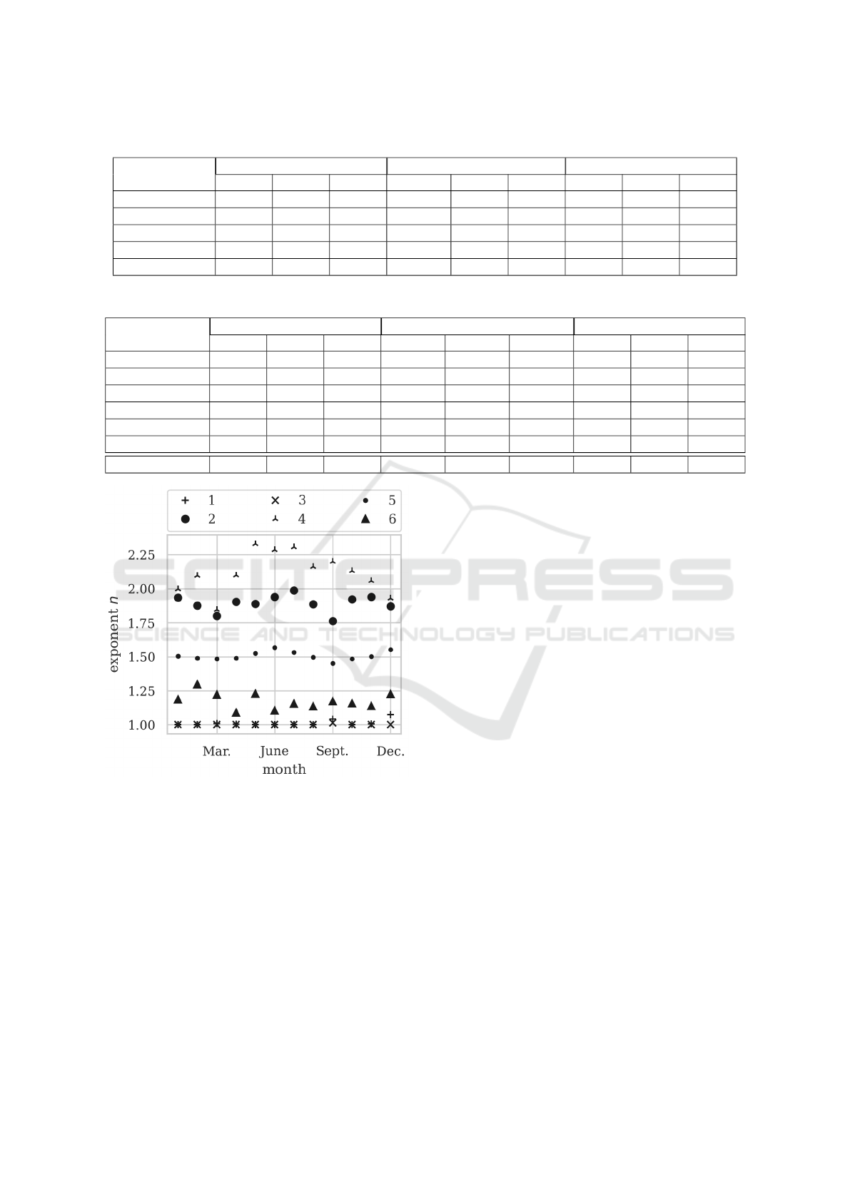
Table 1: Weighted mean RMSE values for each sliding window length.
window length model type I model type II model type III
in weeks set A set B set C set A set B set C set A set B set C
1 5.3303 3.7005 3.7522 9.7823 6.4420 6.3621 5.3288 3.7683 3.7671
2 5.4144 3.8586 3.8769 10.2949 6.5965 6.5028 5.4120 3.9045 3.8830
3 5.4781 3.9986 3.9719 10.5604 6.6956 6.6005 5.4728 4.0093 3.9683
4 5.5352 4.0842 4.0445 10.8248 6.8014 6.7014 5.5310 4.0902 4.0392
5 5.5903 4.1695 4.1236 11.1156 6.9083 6.8011 5.5865 4.1721 4.1163
Table 2: RMSE values for a sliding window of one week.
model type I model type II model type III
air filter set A set B set C set A set B set C set A set B set C
1 6.9818 6.9788 6.9725 10.2139 9.2112 9.2019 7.0094 6.9775 6.9714
2 3.4586 2.9847 2.9725 3.7586 3.0807 3.0660 3.4542 3.0026 2.9900
3 5.5745 5.5556 5.5369 15.6732 13.7007 13.6616 5.5551 5.5554 5.5368
4 3.9553 3.3635 3.3426 4.0731 3.4121 3.4142 3.9408 3.4023 3.4003
5 - 2.3839 2.5264 - 4.8358 4.6676 - 2.5210 2.5311
6 - 2.3471 2.3207 - 2.7927 2.7995 - 2.3959 2.3932
weighted mean 5.3303 3.7005 3.7522 9.7823 6.4420 6.3621 5.3288 3.7683 3.7671
Figure 1: Development of the exponents of model type I.
of model type I. Figure 1 shows that the exponents
of model type I varies around the value of 2 in case
of the return air filters number 2 and number 4. In
contrast, the exponents of the corresponding supply
air filters nearly always have the value 1. Whereas,
the exponents of the supply air filter number 5 are
higher than the exponents of the return air filter num-
ber 6. As shown in Table 2 the quality of fit of the
supply air filters 1 and 3 is worse than the quality of
fit of the corresponding return air filters 2 and 4. This
is also indicated by the values of their exponents. It
was defined that the exponents cannot be lower than
1. So, the fact that the exponents of air filter 1 and
3 mostly have the value 1 also illustrates that a major
influence is lacking in the model for these air filters.
In addition to the differences between the exponents
of each air filter Figure 1 also shows the influence of
the air condition as well as the influence of the build-
ing usage. The analysed building is not that populated
during March, August and September. Therefore, the
HVAC system operates only at partial load or is turned
off during this period. Hence, the amount of samples
decreases and the quality of fit decreases as well. The
influence of the air condition is indicated by a local
maxima during the summer in case of the air filters
2, 4 and 5. In the end this analysis clarifies why the
model type II does not perform as good as the other
models. For this model it is assumed that the expo-
nent has the value 2 which is not the case for each air
filter. The models type I and III offer the possibility to
choose other exponents, in case of model type I and a
mixture of different exponents in case of model type
III. Furthermore, this analysis also illustrates that the
air condition as well as the usage of the building affect
the results of the fit.
6 CONDITION MONITORING
Model type I in combination with set B yields the best
quality of fit. So, the resulting model is used here-
inafter to estimate the condition of air filters. At first
the used condition monitoring method is described
and Section 6.2 contains the results for the dataset
which is described in Section 4.
Condition Monitoring for Air Filters in HVAC Systems with Variable Volume Flow
107
6.1 Method
The model which was selected in Section 5 is used
to estimate the differential pressure at nominal vol-
ume flow
c
∆p
n
. For existing HVAC systems, the dif-
ferential pressure limit is specified for the nominal
volume flow. Thus, the estimated differential pres-
sure at nominal volume flow can be compared with
the already defined differential pressure limit. The es-
timated differential pressure at nominal volume flow
is determined as follows:
1. Start at the beginning of the time series.
2. Define a window of the duration 7 days which se-
lects a data segment.
3. Estimate the variables c and n for the selected data
segment by conducting a least squares fit.
4. Use the air filter model, the determined variables
as well as the measured volume flow and air tem-
perature values to estimate the differential pres-
sure at nominal volume flow for the samples dur-
ing the last day of the selected data segment.
5. Move the window one day further.
6. Repeat the steps 2 to 5 until the time series end.
The estimated differential pressure at nominal volume
flow can be used in two ways. On the one hand, it
can be compared with the specified differential pres-
sure limit and an error message can be returned in
the building management system if the limit is ex-
ceeded. Alternatively, the estimated differential pres-
sure at nominal volume flow can be scaled in such a
way that the resulting value of the filter clogging C
has the value 0% at the initial differential pressure
of the air filter
1
and reaches 100 % when the differ-
ential pressure limit is reached (see Equation 18). In
the analysed building, several air filters from differ-
ent manufacturers are operated in parallel, which is
why the initial differential pressure at the respective
filter stage is unknown. Therefore, in this case the
minimum differential pressure after the filter change
is used as the lower limit.
C =
c
∆p
n
− ∆p
min
∆p
max
− ∆p
min
· 100 % (18)
6.2 Results
The process to determine the air filter condition which
is described in the previous section is applied for each
air filter in the dataset which is described in Section 4.
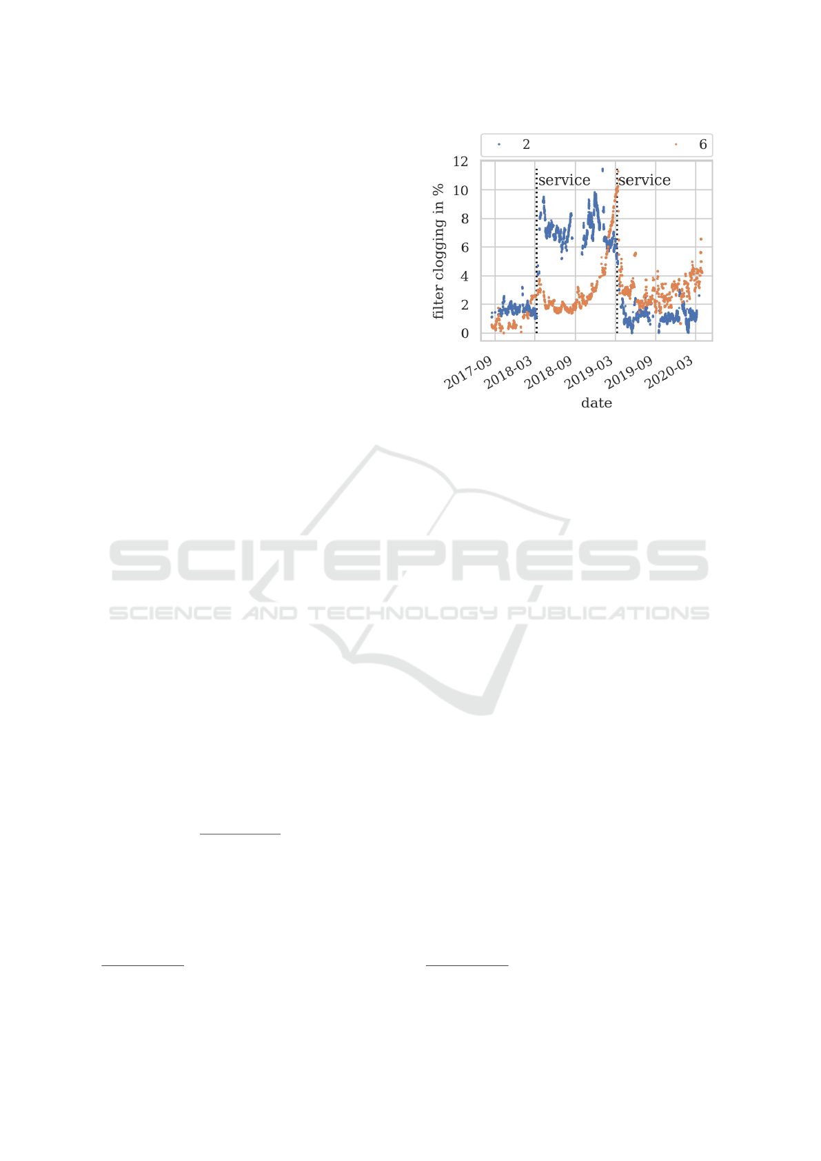
In Figure 2 the results for two air filters are shown
1
The initial differential pressure is usually specified by
the air filter manufacturer.
Figure 2: Filter clogging development for two air filters.
which are representative for all six analysed air filters.
Furthermore, the dates at which the air filters were
changed are marked by the dotted lines
2
.
Figure 2 shows various effects that occur for all air
filters, whereby the strength of the effect varies from
filter to filter. In the case of air filter 6, the reduction
of filter clogging after a filter change is clearly visi-
ble. Whereas in the case of air filter 2, the filter clog-
ging increases after the first service and reduces as
expected after the second service. This effect is a con-
sequence of the use of different air filter brands. Each
air filter brand and type has a different initial differen-
tial pressure, which is why the measured differential
pressure increases after a service and thus also the cal-
culated filter clogging. This effect can be countered
by operating the HVAC system at different volume
flow levels including the nominal volume flow after a
service and using the measured differential pressure at
nominal volume flow as a new lower limit if the initial
differential pressure of the filter brand is not known.
Furthermore, this initial test can be used to determine
the exponent n and keep it fixed until the next service.
This reduces the degrees of freedom of the model and
thus reduces the overfitting potential.
Furthermore, in Figure 2 can be seen that the air
filter clogging for air filter 2 is approximately constant
between each service. This means that the accumu-
lated loading of the air filter with particles between
services has not led to any measurable increase of the
differential pressure at a comparable volume flow. In
addition, the time series shows gaps, as can be seen
for air filter 2 in September 2018 and 2019. These are
2
Due to the COVID-19 pandemic and the lockdown in
Germany no filter change was carried out in March 2020.
SMARTGREENS 2021 - 10th International Conference on Smart Cities and Green ICT Systems
108

caused by the low utilisation of the analysed build-
ing and the associated shutdown of the HVAC system
during this period.
7 CONCLUSIONS
In this work, the approaches for modelling air filters
which are identified in Section 2 are unified in Sec-
tion 3 in such a way that they could be compared with
each other and are also available in different levels of
detail, which are suitable for a retrofit. The model
comparison is carried out on the dataset of a build-
ing in Germany described in Section 4. The compari-
son described in Section 5 shows that the models de-
rived from (DIN Deutsches Institut f
¨
ur Normung e.V.,
2013) and (L
¨
offler, 1988) deliver comparable results.
The former achieves the best results overall. In Sec-
tion 6 is described how this model can be used for
condition monitoring of air filters in HVAC systems
with variable volume flow. In addition, it is shown
that this approach can be retrofitted to an existing
building and provides plausible results.
Nevertheless, following questions with focus on
condition monitoring of air filters in HVAC systems
with variable volume flow are still open for further
research.
• Is it possible to truly increase the quality of the
air filter condition estimation by determining the
exponent of model type I after a filter change and
keeping it fixed for the rest of the air filter life?
• If data with better quality and a higher frequency
resolution in combination with usage of relative
air humidity would be available, how does that af-
fect the performance of the analysed model types?
• Are the results independent from the analysed
building and potential systematic errors in the data
acquisition?
ACKNOWLEDGEMENTS
The authors acknowledge the financial support by the
Federal Ministry for Economic Affairs and Energy
(project number 03ET1569).
REFERENCES
Albers, K.-J., editor (2017). Taschenbuch f
¨
ur Heizung
und Klimatechnik - einschließlich Trinkwasser- und
K
¨
altetechnik sowie Energiekonzepte. DIV Deutscher
Industrieverlag GmbH.
DIN Deutsches Institut f
¨
ur Normung e.V. (2013). Luft-
filtereinlasssysteme von Rotationsmaschinen -
Pr
¨
ufverfahren - Teil 1: Statische Filterelemente (DIN
EN ISO 29461-1:2013). Beuth Verlag GmbH.
Eckhardt, T. (2018). System for Detecting an Air Filter
Condition, in Particular for Combustion Engine (US
10,126,203 B2). United States Patent Office.
Fraden, J. and Rutstein, A. (2007). Clogging Detector for
Air Filter (US 7,178,410 B2). United States Patent
Office.
Kanaoka, C. and Hiragi, S. (1990). Pressure drop of air filter
with dust load. Journal of Aerosol Science, 21(1):127
– 137.
Kang, P., Farzad, M., Stricevic, S., Sadegh, P., and Finn,
A. M. (2007). Technique for Detecting and Predicting
Air Filter Condition (US 7,261,762 B2). United States
Patent Office.
Kang, P., Radeliff, T. D., Farzad, M., and Finn, A. M.
(2006). Method and Control for Testing Air Filter
Condition in HVAC System (US 2006/0130497 A1).
United States Patent Office.
Kruger, A. (2013). The Impact of Filter Loading on Res-
idential HVAC Performance. Master’s thesis, School
of Building Construction, Georgia Institute of Tech-
nology.
Ladusaw, W. T. (1966). Air Filter Condition Indicator (US
3,263,403). United States Patent Office.
L
¨
offler, F. (1988). Staubabscheiden. Georg Thieme Verlag.
Liu, M., Claridge, D. E., and Deng, S. (2003). An air filter
pressure loss model for fan energy calculation in air
handling units. International Journal of Energy Re-
search, 27:589 – 600.
Rivers, R. D. and Murphy, D. J. (2000). Air filter perfor-
mance under variable air volume conditions. Techni-
cal report, American Society of Heating, Refrigerat-
ing and Air-Conditioning Engineers, Inc.
Saarela, O., Hulsund, J. E., Taipale, A., and Hegle, M.
(2014). Remaining useful life estimation for air fil-
ters at a nuclear power plant. In European Conference
of the Prognostics and Health Management.
Verein Deutscher Ingenieure (2004). Filternde Abscheider,
Tiefenfilter aus Fasern (VDI 3677-2:2004-02). Beuth
Verlag GmbH.
Verein Deutscher Ingenieure (2018). Raumlufttech-
nik, Raumluftqualit
¨
at, Hygieneanforderungen an
raumlufttechnische Anlagen und Ger
¨
ate (VDI-
L
¨
uftungsregeln) (VDI 6022-1:2018-01). Beuth Verlag
GmbH.
Condition Monitoring for Air Filters in HVAC Systems with Variable Volume Flow
109
