A Stacking Ensemble-based Approach for Software Effort Estimation

Suyash Shukla and Sandeep Kumar

Department of Computer Science and Engineering, Indian Institute of Technology Roorkee, Roorkee, India

Keywords:

Software Effort Estimation, Machine Learning, Ensemble Models, ISBSG Dataset.

Abstract:

Software Effort Estimation (SEE) is the undertaking of precisely assessing the measure of effort needed to

create software. A lot of exploration has already done in the ﬁeld of SEE using Machine Learning (ML)

strategies to deal with the deﬁciencies of traditional and parametric estimation methodologies and line up with

present-day advancement. Nonetheless, generally due to questionable results and uncertain model develop-

ment strategies, just a few or none of the methodologies can be utilized for deployment. This paper intends

to enhance the procedure of SEE with the assistance of an ensemble based ML approach. So, in this study, a

stacking ensemble-based approach has been proposed for SEE to deal with the previously mentioned issues.

To accomplish this task an International Software Benchmarking Standards Group (ISBSG) dataset has been

utilized along with some data preparation and cross-validation technique. The outcomes of the proposed ap-

proach are compared with Multi-Layer Perceptron (MLP), Support Vector Machine (SVM), and Generalized

Linear Model (GLM) to obtain the best performing model. From the results, it can be concluded that the en-

semble model has produced fewer error estimates contrasted than other models. Lastly, we utilize the existing

approaches as a benchmark and compared their results with the models utilized in this study.

1 INTRODUCTION

SEE is the most challenging activity in software

project management. Earlier, the researchers have

combat a great deal in assessing the perfect measure

of effort or cost. The prediction of these target vari-

ables toward the starting periods of the product lifecy-

cle is increasingly inconvenient because limits for ev-

ery task are needed to set up and the features for the

ﬁnal product are substantial (Boehm, 1981). Inten-

tionally, the expert judgment method that relies on the

information of estimators (Wysocki, 2014) has been

generally utilized in the past. However, these pro-

cedures, for the most part, lead to mistakes; accord-

ingly, different strategies dependent on Line of Code

(LOC) and Function Point (FP) have been presented

previously. The different modiﬁcations of LOC and

FP approaches have also been presented by various

authors to acquire new trends in programming and

software advancement techniques. Although, in the

speedy world of advancement, these techniques are

ﬁghting to stay up with the most recent (Galorath and

Evans, 2006), especially with propelling code reuse

and changed development strategies.

Subsequently, signiﬁcant research has been coor-

dinated to SEE using ML techniques (Sehra et al.,

2017), to deal with the previously mentioned issues.

These strategies are considered especially convinc-

ing for taking care of difﬁculties and the got results

present their unbelievable estimation capacities with

regards to SEE at the initial periods of the lifecy-

cle of the product (Berlin et al., 2009; Tronto et al.,

2008). Nonetheless, generally due to questionable re-

sults and uncertain model development strategies, just

a few or none of the methodologies can be utilized for

deployment. The reason could be the constrained re-

search that focused on ﬁnding the most deﬁnite ML

methodology and ﬁtting it for the best results. Mostly

the obsolete and compact size datasets of completed

software, which are likely to overﬁt have been utilized

in the earlier research (Kocaguneli et al., 2012a). Be-

sides, for data preparation, which is viewed as signif-

icant for making efﬁcient models, distinct, frequently

contradicting methods were applied (Garc

ıa et al.,

2016; Huang et al., 2015). Based on the constraints

portrayed out above, there are unknown results of in-

dividual techniques, whether or not they were exam-

ined on the same dataset. This can be considered as a

consequence of different strategies utilized by experts

for data preparation and creating ML models for SEE.

This paper intends to enhance the procedure of

SEE with the assistance of an ensemble based ML

Shukla, S. and Kumar, S.

A Stacking Ensemble-based Approach for Software Effort Estimation.

DOI: 10.5220/0010405002050212

In Proceedings of the 16th International Conference on Evaluation of Novel Approaches to Software Engineering (ENASE 2021), pages 205-212

ISBN: 978-989-758-508-1

205

approach. Purposefully, we have proposed a stacking

ensemble-based approach to deal with the previously

mentioned issues. To accomplish this task an Interna-

tional Software Benchmarking Standards Group (IS-

BSG) dataset (ISBSG, 2019) has been utilized along

with some data preparation and cross-validation tech-

nique. The outcomes of the proposed approach are

compared to MLP, SVM, and GLM models to obtain

the best performing model. Further, we utilize the ex-

isting approaches as a benchmark and compared their

results with the models utilized in this study. Depend-

ing on the discussion, this paper tries to answer the

following research questions (RQs):

• RQ1: Which model under consideration is pro-

ducing lesser error values for effort estimation?

• RQ2: Whether the heterogeneous nature of data

affecting the performance of the proposed model

or not?

• RQ3: How much improvement/deterioration is

shown by the proposed machine learning model

for effort estimation in comparison to existing

models?

To enquire about these research questions, three indi-

vidual and three ensemble models are created on four

datasets (D1, D2, D3, and D4) for SEE. The datasets

are derived from the ISBSG dataset depending upon

project productivity to deal with the issue of hetero-

geneity. Then, the outcomes of different ML tech-

niques were compared to obtain the best performing

model. Further, the benchmark approaches are con-

trasted with the models utilized in this study.

The remaining paper is organized as follows: Sec-

tion 2 discusses the overview of existing work on

SEE. The methodology used for SEE in this paper

is discussed in section 3. The results obtained uti-

lizing different individual and ensemble models and

statistical analysis have been discussed in section 4

and section 5, respectively. The answers to the re-

search questions are discussed in section 6. Section

7 presents threats related to validity. Finally, the con-

clusion is discussed in section 8.

2 RELATED WORK

The ML strategies have been widely adopted for the

problem of SEE over the last 20 years. The aim was

to predict the effort at the underlying stages since the

estimation toward the starting periods of the product

lifecycle is problematic due to unsure and inadequate

requirements. Any critical deviation of the given in-

formation during the lifecycle of the product may

truly inﬂuence the functionalities of the ﬁnal product,

its standard, and ﬁnally, it’s effective ﬁnishing.

The 84 investigations in which the ML strate-

gies have been used for SEE were explored in (Wen

et al., 2012) to conduct an intensive review. As

showed by the results, the analysts or specialists fo-

cused more on ﬁtting individual algorithms for pre-

cise outcomes, particularly; models dependent on Ar-

tiﬁcial Neural Network (ANN), decision trees, and

Case-Based Reasoning (CBR). They found ML-based

models to be progressively precise contrasted with the

conventional models. They likewise exhibited that de-

pending on the methodologies applied for data prepa-

ration and the dataset used for creating models, the

ML models may prompt complex results.

The irregularity in utilizing different procedures

for creating ML models for SEE is signiﬁcantly per-

ceptible while investigating individual examinations.

For instance, the error estimates of various regression

approaches are analyzed against the ANN model in

(Tronto et al., 2008), displaying the prevalence of the

latter one. In (L

opez-Mart

ın, 2015), they compared

different kinds of ANNs for the problem of SEE uti-

lizing the ISBSG dataset and some data preprocess-

ing. Berlin et al. (Berlin et al., 2009) have also com-

pared the performance of ANN and Linear Regres-

sion (LR) for the effort and duration estimation. They

utilized the ISBSG dataset and along with that, they

used the Israeli Company dataset and found ANN to

be superior to LR. Additionally, they found effort es-

timation to be more precise than duration due to the

high correlation between effort and size.

In (Nassif et al., 2019), they embraced a fuzzy

logic-based regression methodology for SEE. They

ﬁrst performed data preprocessing on the ISBSG

dataset of 6000 projects and obtained a dataset of 468

projects based on their needs. Then, they applied a

fuzzy logic-based regression model and observed that

data heteroscedasticity inﬂuenced the accuracy of ML

models. Also, they found fuzzy logic-based regres-

sion models are reactive to outliers.

Despite various methodologies utilized for devel-

oping ML models, important suggestions that help

their execution practically for SEE at initial project

phases can be taken out. Because of the affectabil-

ity of ML models for outliers inside the data, mod-

els ought not to depend on a single algorithm yet

utilized ensemble, which moreover improves the ac-

curacy (Minku and Yao, 2013). Various ensembles

methods have been proposed by the Analysts, for ex-

ample, bagging, boosting, and stacking (Kocaguneli

et al., 2012b), generally for a similar sort of ML meth-

ods. Nonetheless, these methods may present consid-

erable execution overhead (Azhar et al., 2013) when-

ENASE 2021 - 16th International Conference on Evaluation of Novel Approaches to Software Engineering

206

ever applied in excess. Subsequently, a different set

of simple ensemble algorithms are recommended for

SEE.

The data preparation phase is signiﬁcant in the

model training, especially in the management of out-

liers, the missing information which, to a great extent,

inﬂuences the accuracy of models. Besides the differ-

ent strategies that are accessible for data preparation,

the ML models are generally subject to the dataset

(Huang et al., 2015). In any case, it is prescribed to

use data deletion methods instead of data imputation

for handling missing data because that may decrease

data variability (Strike et al., 2001).

The signiﬁcant difference between this research

and the previous research is that we proposed a stack-

ing ensemble-based method for SEE instead of utiliz-

ing the individual ML models to tackle the issues re-

lated to the outliers in the data. Also, in this study,

we have utilized different datasets, whereas, in the

previous research, only single datasets were consid-

ered for model evaluation. The outcomes of different

ML techniques were compared to obtain the best per-

forming model. Further, the benchmark approaches

are contrasted with the models utilized in this study.

3 PROPOSED APPROACH

This section describes the dataset, procedure used,

different methods used for SEE, and the performance

assessment measures.

3.1 Data Preparation

Noise in the data may truly affect the ML model’s ac-

curacy. The dataset with missing information and out-

liers is viewed as low-quality data. So, data prepara-

tion is a fundamental task during the ML model’s de-

velopment. The ISBSG release 2019 (ISBSG, 2019)

dataset has been utilized to evaluate the ML model’s

performance. According to (Jorgensen and Shepperd,

2007), the quality of SEE investigation can be im-

proved utilizing real-life projects.

3.1.1 Data Filtering

Provided the heterogeneous nature of the ISBSG

dataset and its huge size, a data pre-processing is

needed prior to performing any analysis. The rules

used for data ﬁltering are adapted from (Nassif et al.,

2019). Projects in this study are selected based on the

following characteristics:

• High Data Quality: Each project in the ISBSG

dataset is assigned a data quality rating (A, B, C,

or D). For this study, we have only used projects

with data quality A or B.

• New Development Type: Projects in the ISBSG

dataset are categorized as new development, re-

development, or enhanced development. For this

study, we have considered only newly developed

projects.

• Remove all the projects in which the measurement

for size is other than IFPUG. The IFPUG projects

are selected due to their popularity in the industry.

• No Missing Values for the Development Team

Effort Feature: Remove all the projects with

missing development team effort value.

• No Missing Values for the Development Team

Effort Feature: Projects in the ISBSG dataset are

assigned a productivity value. The productivity

value is a major factor in the effort calculation.

So, we have removed all the projects with missing

productivity value.

3.1.2 Selected Features

Initially, the twenty most frequently used features

have been selected as independent features for ML

models (de Guevara et al., 2016). The eight features

with missing values of more than 60% have been re-

moved from the initial set of 20 features. The Nor-

malized Work Effort Level 1 (NWEL1) is used as a

dependent variable in this study. The resource level

value will be one for all the projects because NWEL1

represents only the development team’s effort. Sim-

ilarly, the development type value will be one for all

the projects because we have considered only newly

developed projects. So, we have removed the resource

level and development type features from the initial

set of features. Hence, the dataset contains only ten

independent variables and one dependent variable.

This study has not used the two features, Applica-

tion Type (AT) and Organization Type (OT). Instead,

their derived versions, Application Group (AG) and

Industry Sector (IS) have been utilized to reduce their

complexity. Finally, the projects having missing val-

ues in any independent variable have been removed

from the dataset. The ﬁnal dataset has 428 projects

with 11 features.

Some of the projects in the dataset are of a simi-

lar size; however, their effort varies. This is due to the

value of the productivity factor (PF), which makes the

data heterogeneous. So, the same model will not pro-

duce good results for all the datasets. Purposefully,

the original dataset is divided into four different sub-

sets by keeping a similar projects together based on

the productivity feature. This will help to tackle the

A Stacking Ensemble-based Approach for Software Effort Estimation

207

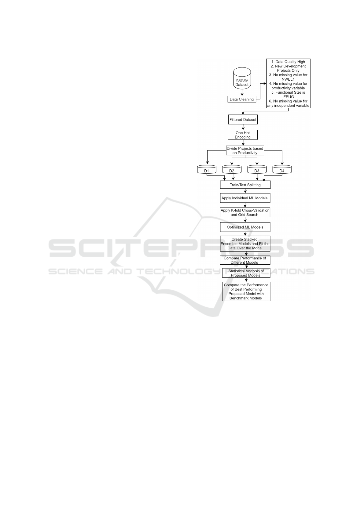
problems that originated from the heterogeneous na-

ture of data. The projects with productivity 0.2 to 10

are in D1. Similarly, projects with productivity 11

to 20 are in D2, whereas projects having productivity

more than 20 are in D3. D4 is the combination of D1,

D2, and D3.

3.2 Methodology

In this study, a stacking ensemble-based approach has

been proposed for SEE to tackle the issues related to

the outliers in the data. The methodology used to cre-

ate stacking ensemble model is shown in Figure 1.

Firstly, we have identiﬁed the top 3 ML methods uti-

lized for SEE research. According to the literature,

the main three ML methods for SEE are MLP, SVM,

and GLM. So, we implemented the models mentioned

above with the help of K-fold cross-validation. Also,

we used a grid search to optimize the parameters of

these models. Then, we created three stacking en-

semble models by considering one model among the

selected three models as a base estimator and the other

two models as meta estimators. So, here we have cre-

ated six different models on four datasets to get accu-

rate effort estimates. The results of these models are

compared to obtain the best performing model. Fur-

ther, the performance of the best performing model is

compared with the benchmark approaches developed

over similar data.

3.3 Stacking Ensemble Model

As referenced above, due to the affectability of ML

models for outliers inside the data, models ought not

to depend on a single algorithm yet utilized ensem-

ble, which moreover improves the accuracy. So, in

this study, we have utilized stacking ensemble mod-

els because of their popularity to provide better re-

sults when combining different models. The stacking

ensemble models are based on the idea of base and

meta estimators (Graczyk et al., 2010). One model

works as a base estimator among the different mod-

els, and the remaining models work as meta estima-

tors. The meta models will be trained on the actual

dataset, whereas the base model will be used on the

meta models’ predictions to improve the accuracy, as

shown in Figure 2.

3.4 Base ML Models used

3.4.1 SVM

In SVM, each project will be considered as the data

point in the n-dimensional space, where n portrays in-

Figure 1: Proposed Methodology for SEE using ML mod-

els.

put variables (Drucker et al., 1997). After that, the es-

timation will be done by recognizing the hyperplane.

The hyperplane will assist us in predicting the effort

value. Here, the fundamental spotlight is on ﬁtting

the value of error inside some limit, whereas the LR

works on the idea of reducing the error.

3.4.2 MLP

The MLP model comprises a minimum of 3 layers; in-

put, hidden, and output (Murtagh, 1991). The number

of hidden layers can be increased with the complex-

ity of the project. The neurons in the input layer are

generally equivalent to the number of features. The

neurons in the output layer rely upon the kind of the

problem. For the regression problem, the neurons in

the output layer are equal to 1. The predicted value

ENASE 2021 - 16th International Conference on Evaluation of Novel Approaches to Software Engineering

208

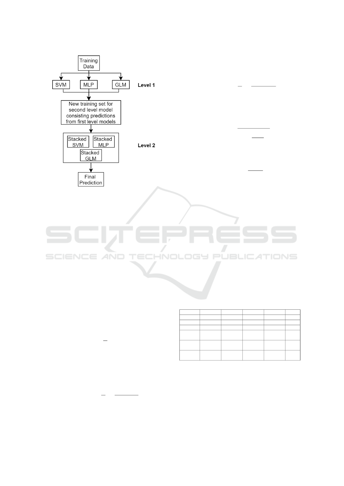
Figure 2: Proposed Stacking Ensemble Model.

will get compared with the actual value, and an error

will be calculated; the focus of the MLP model is to

reduce this error by adjusting model weights.

3.4.3 GLM

GLM models are an extension of the LR model

(Hardin et al., 2007). They can connect the input data

factors based on the output variable and the statisti-

cal properties. They are adaptable, and because of

this quality, they can deal with nonlinear features ef-

fectively. These models are effective for validating

the relation between input and the target variable, and

they also explain the degree to which they are con-

nected.

3.5 Performance Evaluation Measures

• MAE: It is the average of actual and estimated

values (Hardin et al., 2007).

MAE =

∑

i=1

−e

(1)

where, a

= actual values, e

= estimated values,

K= total number of samples.

• MBRE: It is the mean of the absolute error di-

vided by the minimum of actual and estimated

values (Hardin et al., 2007).

MBRE =

∑

i=1

min(a

, e

)

(2)

where,

−e

(3)

• MIBRE: It is the mean of the absolute error di-

vided by the maximum of actual and estimated

values (Hardin et al., 2007).

MIBRE =

∑

i=1

max(a

, e

)

(4)

• RMSE: It is calculated by taking the square root

of the mean of squared differences between actual

and estimated values (Satapathy and Rath, 2017).

MSE =

∑

i=1

−e

)

(5)

RMSE =

√

MSE (6)

• SA: It is calculated by taking the ratio of MAE

and MAE

(Azzeh and Nassif, 2016).

SA = 1 −

MAE

(7)

MAE

will be obtained by predicting the value

for the query utilizing many random sampling

runs over the remaining K-1 cases.

4 RESULTS

In this research, a stacking ensemble-based approach

is utilized to improve the performance of SEE as the

individual models are reactive to the outliers. The re-

sults of different models for datsets D1, D2, D3, and

D4 are shown in Table 1- 4.

For dataset D1, the Stacked-SVR is performing

well compared to the other models in terms of MAE

and RMSE, whereas in terms of MBRE and MIBRE,

the best performing models are Stacked-GLM and

Stacked-MLP, respectively.

Table 1: Error measures for effort estimation on dataset D1.

MAE MBRE MIBRE RMSE SA

SVM 911.2565 0.975362 0.375842 1619.643 81.04

MLP 989.9004 1.237125 0.354877 1685.743 79.41

GLM 993.4792 0.891887 0.734239 1700.488 79.33

Stacked-

GLM

1672.262 0.051911 1.715548 2674.172 65.21

Stacked-

SVM

898.9615 1.025823 0.383532 1596.473 81.30

Stacked-

MLP

1007.73 1.072949 0.341323 1762.341 79.03

For dataset D2, the Stacked-GLM has outper-

formed all the other models for every measure in the

case of dataset D2.

The Stacked-SVR model performs well compared

to the other models for dataset D3 in terms of most of

the measures. Similarly, for dataset D4, the Stacked-

MLP model is performing well compared to the other

models in terms of MAE and MIBRE.

A Stacking Ensemble-based Approach for Software Effort Estimation

209

Table 2: Error measures for effort estimation on dataset D2.

MAE MBRE MIBRE RMSE SA

SVM 959.028 0.196013 0.15525 1454.975 81.83

MLP 1148.351 0.295753 0.203993 1652.75 78.24

GLM 938.0946 0.317627 0.197054 1288.577 82.22

Stacked-

GLM

875.8321 0.193439 0.152351 1282.26 83.40

Stacked-

SVM

1030.827 0.212693 0.166407 1566.16 80.46

Stacked-

MLP

1167.427 0.248622 0.181989 1814.745 77.88

Table 3: Error measures for effort estimation on dataset D3.

MAE MBRE MIBRE RMSE SA

SVM 3408.197 0.424001 0.241235 7789.522 70.31

MLP 3887.964 0.505984 0.284849 7153.903 66.13

GLM 3793.644 0.484938 0.281544 7049.025 66.95

Stacked-

GLM

3851.727 0.521349 0.286092 7199.061 66.45

Stacked-

SVM

3390.099 0.414885 0.236534 7786.483 70.47

Stacked-

MLP

3415.554 0.42173 0.243809 7714.72 70.25

Table 4: Error measures for effort estimation on dataset D4.

MAE MBRE MIBRE RMSE SA

SVM 4240.309 2.882393 0.543553 7526.181 38.93

MLP 3614.042 1.921557 0.492598 5390.022 47.95

GLM 3205.317 1.997729 0.471746 4756.324 53.84

Stacked-

GLM

3273.134 0.329232 1.00303 5253.333 52.86

Stacked-

SVM

4278.489 2.952899 0.547017 7575.351 38.38

Stacked-

MLP

2965.281 1.551779 0.431978 4804.453 57.29

5 STATISTICAL ANALYSIS

5.1 Comparison of Models

In this subsection, a Wilcoxon test (Han et al., 2006)

is conducted, which inspects the similarity or dissimi-

larity of the two distributions based on the hypothesis:

: No signiﬁcant difference among the two

models P1 and P2

: The two models P1 and P2, are signiﬁcantly

different

The hypothesis relies on the p-value, i.e., a p-value

greater than 0.05 suggests the acceptance of H0,

whereas a p-value greater than 0.05 shows the re-

jection of H0. The p-values for the Stacked-SVR,

Stacked-MLP, and Stacked-GLM models for different

datasets are shown in Table 5- 7.

The p-values for the Stacked-SVR model show

that the null hypothesis is accepted for most of the

models over the four datasets, as shown in Table 5.

Table 5: Wilcoxon test result for Stacked SVR model.

D1 D2 D3 D4

SVM 0.000 0.061 0.000 0.000

MLP 0.974 0.000 0.000 0.000

GLM 0.708 0.989 0.000 0.000

Stacked-GLM

0.000 0.000 0.000 0.000

Stacked-MLP

0.000 0.009 0.000 0.000

Table 6: Wilcoxon test result for Stacked MLP model.

D1 D2 D3 D4

SVM 0.000 0.000 0.000 0.000

MLP 0.0031 0.000 0.000 0.000

GLM 0.000 0.000 0.000 0.000

Stacked-GLM

0.000 0.000 0.000 0.000

Stacked-SVM

0.000 0.000 0.000 0.487

From Table 6, it is clear that the p-values for the

Stacked-MLP model suggest the acceptance of the

null hypothesis for all the models except the Stacked-

SVR model for D4.

Table 7: Wilcoxon test result for Stacked GLM model.

D1 D2 D3 D4

SVM 0.000 0.019 0.000 0.000

MLP 0.000 0.000 0.000 0.000

GLM 0.000 0.090 0.000 0.000

Stacked-SVM

0.000 0.009 0.000 0.000

Stacked-MLP

0.000 0.000 0.000 0.487

Similar to Stacked-MLP, the p-values for the

Stacked-GLM model also favor the null hypothesis

for all the models over all the datasets except Stacked-

MLP for D4, as shown in Table 7.

5.2 Comparison with Benchmark

Models

In this subsection, the benchmark approaches are con-

trasted with the different ensemble models utilized

in this study based on the MAE measure. In (Nas-

sif et al., 2019), Multiple Linear Regression (MLR)

and Fuzzy models were implemented, and their per-

formance was compared with the ANN model. We

have also compared the performance of models uti-

lized in this study against the best performing model

in (Nassif et al., 2019) and the ANN model, which is

shown in Table 8.

Table 8 shows that the stacking ensemble-based

models are performing well for different datasets. For

datasets D1 and D3, Stacked-SVR performs well,

whereas, for D2 and D4, Stacked-GLM and Stacked-

MLP are performing well, respectively.

ENASE 2021 - 16th International Conference on Evaluation of Novel Approaches to Software Engineering

210

Table 8: Comparison of the proposed model with bench-

mark models based on different measures.

D1 D2 D3 D4

Stacked GLM

1672.262 875.8321 3851.727 3273.134

Stacked SVR

898.9615 1030.827 3390.099 4278.5

Stacked MLP

1007.73 1167.427 3415.554 2965.3

ANN Model

(Nassif et al., 2019)

1842.61 1342.3 7241.36 4925.23

Fuzzy Model

(Nassif et al., 2019)

2041.65 3208.02 8499.06 5654.99

MLR Model

(Nassif et al., 2019)

1518.4 1418.6 4742.1 3982

6 DISCUSSION

The answers to the research questions have been given

in this section:

RQ1: Which model under consideration is producing

lesser error values for effort estimation?

To answer this RQ, we proposed a stacking ensemble-

based method for SEE and utilized four different

datasets and ﬁve accuracy measures to evaluate these

models’ performance. Table 1-4 displays the out-

comes of these measures on applying the above-

mentioned ML models over the datasets D1, D2, D3,

and D4, respectively. Based on the observations, we

can say that the proposed stacking ensemble models

are performing well for SEE.

RQ2: Whether the heterogeneous nature of data af-

fecting the performance of the proposed model or

not?

To answer this question, we have divided the origi-

nal ISBSG dataset into four different datasets based

on their productivity values. D1 and D2, which are

mostly homogeneous datasets and contain smaller

productivity range projects are producing fewer error

estimates than the dataset D3 and D4. The dataset

D3 contains projects with productivity values in the

range of 20 to more than 168. Due to the wide range

of productivity, this data is not completely homoge-

neous similar to dataset D4.

RQ3: How much improvement/deterioration is shown

by the proposed machine learning model for effort es-

timation compared to existing models?

To answer this RQ, we utilize the existing approaches

as a benchmark and compared their results with the

models utilized in this study. The error estimates of

existing approaches, along with the proposed models,

are displayed in Table 9. The percentage of improve-

ment/deterioration of the proposed stacking ensemble

models for SEE compared to existing models is cal-

culated based on MAE values and shown in Table 9.

From Table 9, we can say that the proposed model

has shown a lot of improvement in the error values;

the best performing model has improved the perfor-

Table 9: Benchmark vs. proposed model comparison based

on MAE measure.

D1 D2 D3 D4

Benchmark

Model

1518.4

(MLR)

1418.6

(MLR)

4742.1

(MLR)

3982

(MLR)

Proposed

Model

898.96

(Stacked

SVR)

875.8321

(Stacked

GLM)

3390.099

(Stacked

SVR)

2965.3

(Stacked

MLP)

Improvement/

Deterioration

40.79%

(imp)

38.26%

(imp)

28.51%

(imp)

25.53%

(imp)

mance by 40.79%, 38.26%, 28.51%, and 25.53% for

the datasets D1, D2, D3, and D4, respectively.

7 THREATS TO VALIDITY

The threats related to validity are described following:

Internal Validity: As detailed during data prepara-

tion, the ISBSG dataset contains projects whose size

is given in terms of FPs. Here also, the projects

with size measures other than IFPUG are ﬁltered.

Nonetheless, there is a need to explore projects with

different sizing measures. However, this is challeng-

ing as reliable, and good quality data is not easily ac-

cessible.

External Validity: It queries the generalization of re-

sults. Three different stacking ensemble models are

explored in this study over the ISBSG dataset utiliz-

ing some data preparation. The ﬁve measures are used

to evaluate the performance of these models. Further,

we utilize the Wilcoxon test to inspect the validity of

the proposed model. So, the prediction results are

generalized. However, they can still be improved uti-

lizing several other datasets.

8 CONCLUSIONS

This paper intends to enhance the procedure of SEE

with the assistance of an ensemble based ML ap-

proach. Purposefully, we have proposed a stacking

ensemble-based approach to deal with the previously

mentioned issues. To accomplish this task, an IS-

BSG dataset has been utilized along with some data

preparation and cross-validation technique. After per-

forming data preprocessing, only 428 projects were

left in the dataset. The dataset has then been di-

vided into four different subsets by keeping a simi-

lar type of project together. The four datasets have

been provided as input to the proposed models, and

the got outcomes are compared to obtain the best per-

forming model. From the results, it has been found

that the different stacking ensemble-based models are

performing well for different datasets. The Stacked-

A Stacking Ensemble-based Approach for Software Effort Estimation

211

SVR has emerged as the best model for datasets D1

and D3, whereas, for D2 and D4, Stacked-GLM and

Stacked-MLP are the best performing models, respec-

tively. The results are then validated with the help

of p-values. The best performing ensemble model

has been compared with the benchmark models; the

best performing model has improved the performance

by 40.79%, 38.26%, 28.51%, and 25.53% for the

datasets D1, D2, D3, and D4, respectively.

REFERENCES

Azhar, D., Riddle, P., Mendes, E., Mittas, N., and Angelis,

L. (2013). Using ensembles for web effort estimation.

In ACM/IEEE International Symposium on Empirical

Software Engineering and Measurement, pages 173–

182.

Azzeh, M. and Nassif, A. (2016). A hybrid model for es-

timating software project effort from use case points.

Applied Soft Computing, 49:981–990.

Berlin, S., Raz, T., Glezer, C., and Zviran, M. (2009). Com-

parison of estimation methods of cost and duration in

it projects. Information and software technology jour-

nal, 51:738–748.

Boehm, B. W. (1981). Software Engineering Economics.

Prentice Hall, 10 edition.

de Guevara, F. G. L., Diego, M. F., Lokan, C., and Mendes,

E. (2016). The usage of isbsg data ﬁelds in software

effort estimation: a systematic mapping study. ournal

of Systems and Software, 113:188–215.

Drucker, H., Burges, C., Kaufman, L., Smola, A., and Vap-

nik, V. (1997). Support vector regression machines.

In In Advances in neural information processing sys-

tems, pages 155–161.

Galorath, D. and Evans, M. (2006). Software Sizing, Es-

timation, and Risk Management. Auerbach Publica-

tions.

Garc

ıa, S., Luengo, J., and Herrera, F. (2016). Tuto-

rial on practical tips of the most inﬂuential data pre-

processing algorithms in data mining. Knowledge

based Systems, 98:1–29.

Graczyk, M., Lasota, T., Trawi

nski, B., and Trawi

nski, K.

(2010). Comparison of bagging, boosting, and stack-

ing ensembles applied to real estate appraisal. In Asian

conference on intelligent information and database

systems, pages 340–350.

Han, J., Kamber, M., and Pei, J. (2006). Data Mining: Con-

cepts and Techniques. Morgan Kaufmann.

Hardin, J., Hardin, J., Hilbe, J., and Hilbe, J. (2007). Gen-

eralized linear models and extensions. Stata press.

Huang, J., Li, Y., and Xie, M. (2015). An empirical anal-

ysis of data preprocessing for machine learning-based

software cost estimation. Information and Software

Technology, 67:108–127.

ISBSG (2019). International Software Benchmarking Stan-

dards Group.

Jorgensen, M. and Shepperd, M. (2007). A system-

atic review of software development cost estimation

studies. IEEE Transaction of Software Engineering,

33(1):33–53.

Kocaguneli, E., Menzies, T., and Keung, J. (2012a). On the

value of ensemble effort estimation. IEEE Transaction

of Software Engineering, 38:1402–1416.

Kocaguneli, E., Menzies, T., and Keung, J. (2012b). On the

value of ensemble effort estimation. IEEE Transaction

of Software Engineering, 38:1402–1416.

opez-Mart

ın, C. (2015). Predictive accuracy comparison

between neural networks and statistical regression for

development effort of software projects. Applied Soft

Computing, 27:434–449.

Minku, L. and Yao, X. (2013). Ensembles and locality: In-

sight on improving software effort estimation. Infor-

mation and Software Technology, 55(8):1512–1528.

Murtagh, F. (1991). Multilayer perceptrons for classiﬁ-

cation and regression. Neurocomputing, 2(5-6):183–

197.

Nassif, A., Azzeh, M., Idri, A., and Abran, A. (2019). Soft-

ware development effort estimation using regression

fuzzy models. Computational intelligence and neuro-

science.

Satapathy, S. and Rath, S. (2017). Empirical assessment of

ml models for effort estimation of web-based appli-

cations. In In Proceedings of the 10th Innovations in

Software Engineering Conference, page 74–84.

Sehra, S., Brar, Y., Kaur, N., and Sehra, S. (2017). Research

patterns and trends in software effort estimation. In-

formation and software technology journal.

Strike, K., Emam, K., and Madhavji, N. (2001). Software

cost estimation with incomplete data. IEEE Transac-

tion of Software Engineering, 27:890–908.

Tronto, I., Silva, J., and Anna, S. (2008). An investigation

of artiﬁcial neural networks based prediction systems

in software project management. Journal of Systems

and Software, 81:356–367.

Wen, J., Li, S., Lin, Z., Hu, Y., and Huang, C. (2012). Sys-

tematic literature review of machine learning based

software development effort estimation models. In-

formation and Software Technology, 54:41–59.

Wysocki, R. (2014). Effective Project Management: Tradi-

tional, Agile, Extreme, Industry Week. John Wiley &

Sons.

ENASE 2021 - 16th International Conference on Evaluation of Novel Approaches to Software Engineering

212