An Intelligent Transportation System for Air and Noise Pollution
Management in Cities
Mariam Osama Zaky and Hassan Soubra
Department of Computer Science and Engineering, German University in Cairo, Cairo, Egypt
Keywords:
IoT, ITS, Smart Cities, Air and Noise Pollution, Vehicle Routing.
Abstract:
Air quality and noise levels in urban cities have become major environmental concerns worldwide. Road
vehicles are a primary source of air pollution in urban cities and they also are a considerable source of noise
pollution. Undeniably, air and noise pollution are hazardous to human health. Managing pollution levels has
become an absolute priority in order to reduce the anthropogenic impact on the environment. In this paper, we
propose an Intelligent Transportation System-ITS for monitoring and managing air and noise pollution caused
by road vehicles in cities. The system proposed dynamically routes a vehicle using, on the one hand, its
particle emissions and noise indicators; and on the other hand, a city’s pollution levels and defined thresholds.
The system proposed in this paper could be used for pollution based road tolls or taxes.
1 INTRODUCTION
Road vehicles, commonly known as cars, allow ease
of mobility and hence their usage has become es-
sential for people. Due to the dramatic growth in
the world’s population and car ownership, hence, the
number of cars roaming the roads have increased.
Currently the world population is increasing with a
rate of 1.05%, which is estimated to be 81 million
people per year (Worldometer, 2020). And based on
the statistics done by the International Organization
of Motor Vehicle Manufacturers (OICA), sales of ve-
hicles have increased from 66 million units in 2005 to
91 million in 2019, including both passenger cars and
commercial vehicles (IOMVM, 2019).
The increase in the number of vehicles on the
roads has many consequences on the environment
and notably on people. First off, there is an obvi-
ous increase in traffic congestion: rush hours have
become irregular and, hence, unpredictable. Traffic
congestion is related to the difference between the
road traffic performance and its actual condition. In
other words, congestion happens when the number
of vehicles present on a particular road at the same
time exceeds its capacity. Generally, traffic conges-
tion has negative effects on the economy because of
time wastage, but it also has a negative effect on
fuel consumption -which in turn causes gas emis-
sion and air pollution, noise pollution, and finally on
vehicle wear and tear and on road safety (C P and
Karuppanagounder, 2018). The delays caused by con-
gestion make drivers waste a lot of time leading to
late arrivals to work and possibly missing important
meetings; and more importantly delays in delivery of
goods often causing customer dissatisfaction. Hence,
traffic congestion impacts the economy.
Traffic congestion makes cars stop and start many
times, leading to more fuel consumption than cars that
travel without stopping. Based on a study done in
Slovenia in 2018, it has been found that fuel consump-
tion during acceleration was 2.65 times more than the
average fuel consumption (Jereb et al., 2018).
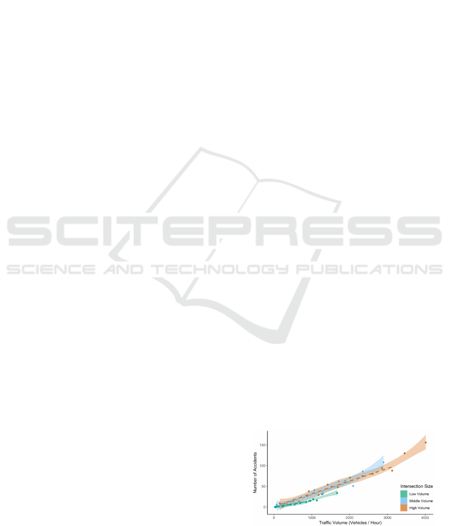
In addition, the number of road traffic accidents
is highly correlated to the number of cars (Figure
1). The World Health Organisation stated that around
1.35 million people die yearly because of road acci-
dents, and many more suffer from dangerous injuries
(WHO, 2020).
Moreover, the environment, and in consequence
humans, are also affected. The increase in usage of
Figure 1: Relationship between traffic volume and accident
frequency (Retallack and Ostendorf, 2020).
Zaky, M. and Soubra, H.
An Intelligent Transportation System for Air and Noise Pollution Management in Cities.
DOI: 10.5220/0010403403330340
In Proceedings of the 7th International Conference on Vehicle Technology and Intelligent Transport Systems (VEHITS 2021), pages 333-340
ISBN: 978-989-758-513-5
Copyright
c
2021 by SCITEPRESS – Science and Technology Publications, Lda. All rights reserved
333
cars and their omnipresence led to extremely high
pollution rates inside cities. For example, The Min-
istry of State for Environmental Affairs of Egypt esti-
mates that vehicle emissions represent about 26% of
total pollution caused by suspended particulate mat-
ter (PM10) in Greater Cairo, 90% of carbon monox-
ide (CO) and 50% of nitrogen oxides (NOx) (Abou-
Ali and Thomas, 2011). Transportation systems -
including cars- are also responsible for around 25% of
Carbon Dioxide (CO2) emissions in the world (BBC,
2020). CO2 is one of the Greenhouse Gases. Green-
house Gases have an extremely dangerous effect on
the ozone layer of our planet. They lock in the heat
causing climate change, notoriously also known as
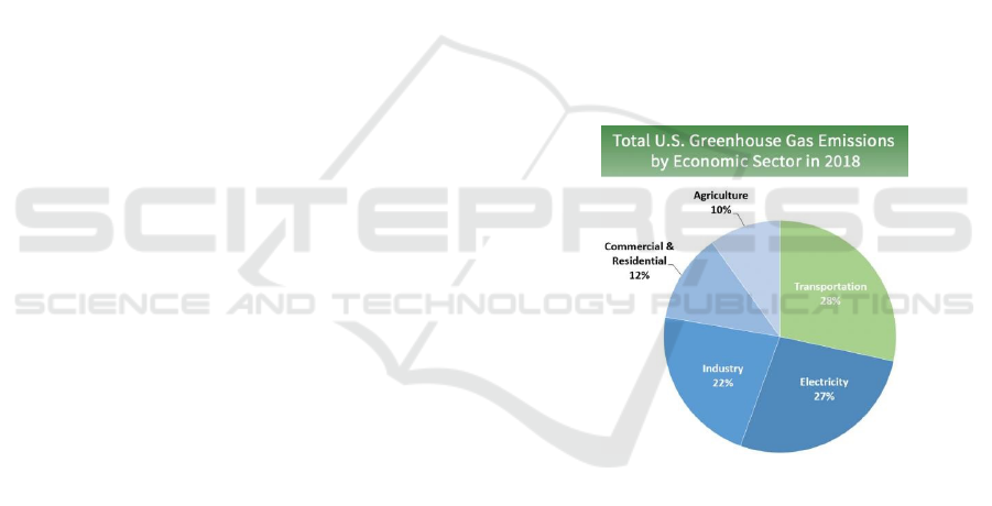
Global Warming (USEPA, 2018). In 2018, trans-
portation was considered the largest source of Green-
house Gases in the United States with a contribu-
tion of 28.2% of the emissions as shown in Figure
2 (USEPA, 2018).
Naturally, inhaling the particles from vehicles’
emissions also have a harmful, and sometimes deadly,
effect on human health and other living beings. A re-
port of the government of Canada (2019) states that
the exposure to air pollution causes lung related dis-
eases, such as asthma and allergies, in addition to
heart related diseases e.g. hypertension, heart attack,
and heart failure. Moreover, the report concluded
that more than 14,000 premature deaths per year in
Canada can be linked to air pollution (Canada, 2019).
Air pollution is one part of the equation, the sec-
ond part lies in the amount of noise pollution. There
are several sources of noise pollution in a vehicle:
noise could stem from its engine, especially if it is
old and does not get proper maintenance; squealing
brakes; different resonating parts; etc. In addition, a
car has human controlled noise sources such as: the
probable excessive use of the car’s horn, the use of
high-volume radio and music systems, etc.
According to the conclusions of the Environmen-
tal Burden of Disease report by the World Health Or-
ganization, noise pollution is ranked the second en-
vironmental threat in Europe after the air pollution
(WHO, 2011).
Noise pollution has several negative impacts on
human health. Noise causes emotional and behav-
ioral stress. An exposure to a sudden loud noise may
cause severe damage to the eardrum and may lead to
hear loss. It can also cause headaches, high blood
pressure, and heart failure (Subramani et al., 2012).
Moreover, noise is the major cause of sleeplessness
and sleep disturbance; psychological disorders; hy-
peractivity and learning difficulties in children; as
well as fatigue and reduced productivity (Wokekoro,
2020). The European Environment Agency estimates
that around 10,000 people die prematurely every year
because of their exposure to noise pollution (EEA,
2020).
Thus, noise stemming from cars should also be
managed and reduced as much as possible.
Road traffic cars are hence considered to be the main
contributor to both air and noise pollution. Approv-
ingly, the World Health Organization (WHO) states
that both air and noise pollution are the most harmful
environmental problems (EEA, 2019).
In this study we aim at monitoring and minimiz-
ing car air and noise pollution inside urban cities. Our
approach is to implement an IoT system consisting
of a network of sensors embedded inside the car to
monitor, in real-time, its particle emissions and noise
level. An additional network of sensors embedded in
the city’s infrastructure is also used in our system in
order to obtain its pollution levels in real-time.
This paper is divided as follows: section 2
presents the literature review. While section 3 de-
scribes the pollution ITS proposed, section 4 dis-
cusses the experiment process and the results. Finally,
a conclusion follows in section 5.
Figure 2: Sources of Green-house Gases in the United
States (USEPA, 2018).
2 LITERATURE REVIEW
In this section, the literature review is presented and
discussed. Several research works on how to monitor
and control vehicles pollution are summarized in this
section.
(Kumar, 2017) claims that cars’ emissions cannot
be 100% prevented unfortunately. Nevertheless, they
can be monitored and controlled in order to reduce
them as much as possible to decrease their harmful
effects. The amount of harmful emissions is directly
proportional to the car’s age and usage. Also, they
depend on whether the car gets maintenance properly
and on a regular basis or not.
VEHITS 2021 - 7th International Conference on Vehicle Technology and Intelligent Transport Systems
334

Noise is measured in Decibels-dB using sound sen-
sors or sound level meters. However, measuring noise
levels produced from a specific source is challenging,
because the noise signals produced from the intended
source are affected by the background and the sur-
rounding noises. Hence, the noise sensors read inac-
curate values (Subramani et al., 2012).
2.1 Air Pollution
A sensor node was implemented by (Miralavy et al.,
2019) on the car’s exhaust system to monitor its emis-
sions. They then sent the sensed data along with the
car’s information to a base station that is controlled
by the authorities. If the car’s pollution level exceeds
a certain limit, the authorities should warn the car
owner to fix it. And if the problem persists, the car
owner would be charged.
(Kundu and Maulik, 2020) implemented a system
which detects pollutant vehicles using deep learning
techniques on real-time images of the vehicles. These
images are captured from the infrastructure or from
neighboring vehicles. They used the Inception-V3
model, which is an image recognition model provided
by Google. After training and testing their model,
they achieved 97% accuracy in the unknown testing
data set. This model depends on the shape and color
of the vehicle’s exhaust. However, some pollutant
emissions are transparent and cannot be seen or de-
tected by images. This model will not be able to de-
tect such types of emissions.
Another study (Muthumurugan, 2018) focused on
measuring light, air, noise, and thermal pollution of
vehicles by connecting suitable sensors to a micro-
controller. When the sensors read data exceeding the
allowed limit, the vehicle will send a message to the
control room within the area, through a GSM module,
and displays the message to the vehicle’s owner with
the phone number of the nearest service center, so ap-
propriate service is provided to fix possible issues .
An MQ-135 gas sensor was used by (Reshi et al.,
2013) to sense NOx, Benzene, and CO2. And an MQ-
7 sensor to measure CO. Then they sent the data to
the server using GPRS (in the form of SMS), based
on 2G/3G communication networks. The data gets
uploaded then to a database and is used to inform
or alert the car owner about the respect of pollution
thresholds.
(Dhingra et al., 2019) implemented a sensor net-
work in specific locations around the city. These sen-
sors collect data about the air pollution level. Firstly,
they collect the data from the sensors that are con-
nected to an Arduino board. The Arduino board sends
then these readings to a cloud platform to store them.
The Arduino board uses a Wi-Fi module to connect to
the internet. When the driver enters the source and the
destination of a the journey, the system gets the route
between them using Google Maps Routing API, then
predicts the pollution level of the entire route and send
warnings to the user if the pollution level is too high,
so the driver can reroute their car. The system also
keeps track of the history of the predictions.
Another study by (Guanochanga et al., 2019) im-
plements a wireless network with gateway nodes that
have internet access and sensor nodes. The sensor
nodes send the air pollution measurements to the cor-
responding gateway node. Then, the data is sent to
a cloud server via the gateway node. After that, it
will be published on a web page that is available for
the users and accessible using web browsers or smart-
phones.
2.2 Noise Pollution
Measuring traffic noise is complicated because it is in-
fluenced by many attributes: Traffic density, vehicles
velocity, traffic flow, road surface type and condition,
vehicle mass, tires, road inclination, etc. All these
attributes are not constant. Therefore, traffic noise
power constantly varies in time and space (Prezelj and
Murovec, 2017).
(Afsharnia et al., 2016) used a TES sound meter
to measure the traffic noise level in the city of Bir-
jand in Iran. the objective of this study is to com-
pare the noise pollution level in Birjand with national
standard-levels. The TES sound meter is used to mea-
sure daily sound levels at several stations and during
four different time periods: morning, noon, evening
and night. The average results of the measurements is
78.1db in the morning, 82.25db in the noon, 81.21db
in the evening, and 81.01db in the night. The study
concluded that generally morning has lower noise lev-
els than noon, and evening is also quieter than night.
In (Fiedler and Zannin, 2015) researchers aimed
to examine the environmental impact of road traffic
noise in the city of Curitiba, Brazil. Their object is
the main urban traffic hubs. They used B&K 2238
and B&K 2250 sound analyzers for noise level mea-
surements, and predictor 8.11 software for acoustic
map calculations. They measured the noise level in
232 different points. 171 of these points showed noise
levels exceeding 65db which is the maximum sound
level people can hear safely and which is extremely
dangerous. The researchers introduced three hypo-
thetical scenarios in attempt to reduce the noise lev-
els. The first scenario simulates reducing the current
total number of vehicles by 50%. The second one
simulates reducing 50% of the heavy vehicles in the
An Intelligent Transportation System for Air and Noise Pollution Management in Cities
335
traffic hubs. Finally, the third one simulates a 56%
increase in the total number of vehicles in traffic over
the next 10 years. The results of the first two scenar-
ios showed a decrease of 3db of the calculated noise
level. On the other hand, the third scenario resulted in
a 3db increase in the noise level.
Moreover, a study by (Ballesteros et al., 2015) fo-
cused on figuring out the noise source of a pass-by
car. The authors wanted to prove that Beam forming
is able to identify the noise sources of a moving car
and get more insight to the mechanisms of the gener-
ated noise. They used a planar 56-microphone array
with 28 additional microphones, located on 8 exter-
nal arms attached to the center array, they also limited
the measurement area with two light barriers. From
the generated noise source maps, they concluded that
the noise is mainly located near the center of the car
tread, and it is slightly louder in the front tires than in
the back ones.
A study by (Desarnaulds et al., 2004) in Sweden
stated that when a car’s speed is reduced from 50km/h
to 30km/h, its noise decreases by 2 to 4dB. Similarly,
in Delft and in Oslo respectively, two studies (Lopez-
Aparicio et al., 2020) (den Boer and Schroten, 2007)
analyzed the effect of reducing the traffic speed limit
on the traffic noise levels. Both studies showed that
reducing traffic speed limit has an effective result in
reducing the noise pollution caused by cars.
After analysing the scientific literature, and to our
best knowledge, there are no intelligent transportation
systems that aim at reducing air and noise pollution in
urban cities via routing decisions based on predefined
city entry-exit points in a addition to pollution indi-
cators, fixed thresholds, and real-time pollution level
readings from both the vehicle and the city sides.
3 PROPOSED POLLUTION
MANAGEMENT ITS
The system proposed measures, in real-time, the cur-
rent air and noise pollution levels of the car and of the
city using IoT sensors embedded in both the car and
the infrastructure. Using the car’s current location and
its destination, the system determines the most effi-
cient route according to the measured pollution levels
and their effect on the ongoing city pollution levels.
The system is divided into two layers: software and
hardware. The software layer includes two different
parts: the server side which is managed by an admin;
and the user side which informs the driver about the
pollution levels and the route. The hardware part con-
sists of a network of wireless sensors embedded in the
car and in the city’s infrastructure.
3.1 Software Implementation
3.1.1 Server Side
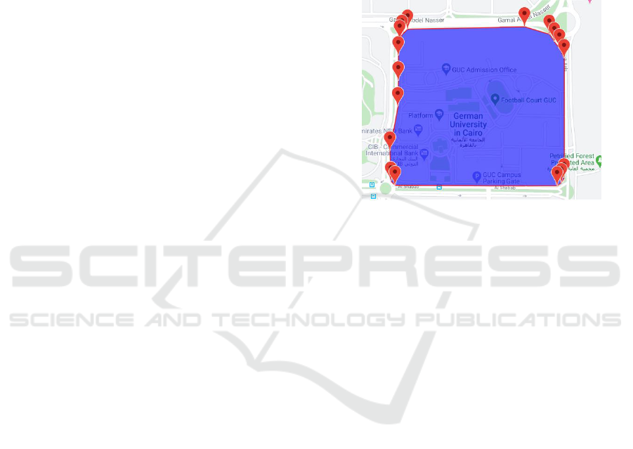
The server is considered to be the back-end of the
application. It is responsible for defining the city’s
information. The city information includes: its bor-
ders, the geographical locations of its different en-
trance and exit points, its pollution thresholds, and its
name e.g. see Figure 3.
Figure 3: Representation of a city showing its borders and
its different entry-exit points as defined on the server.
The city’s information will then be used to set the
routing rules for the vehicles entering and exiting the
city, based on the origin-location and destination of
the user. The Vehicle’s origin and destination points
play a role in deciding whether it will be subjected to
the routing technique proposed to reduce the pollution
rate inside the city or not. If the Vehicle’s origin and
destination points are inside the boundary of one of
the defined cities in the database, the vehicle’s pollu-
tion levels are then taken into consideration with that
city pollution thresholds and current pollution rate.
Next, the system generates two routes: 1-a pollution
optimized route, which cares for reducing the amount
of pollution produced inside the city; 2-and the over-
all shortest path based on Google Maps routing API.
The system also calculates the total distance that the
car will travel in both routes. The two routes are then
displayed to the user through an application.
The back-end is connected to a database contain-
ing the information about the registered cars. Each
registered car gets an identifier that represents a
unique ID (UID) for the car, and has: a model infor-
mation about its make and year of production, a plate
number, and a toll credit. When retrieving the data of
a car, the server also gets the nominal average amount
of gas emission of that car type. The server retrieves
this information from the official website of the U.S
government for fuel company using the car’s model
and year of production (Fueleconomy.gov, 2020).
VEHITS 2021 - 7th International Conference on Vehicle Technology and Intelligent Transport Systems
336
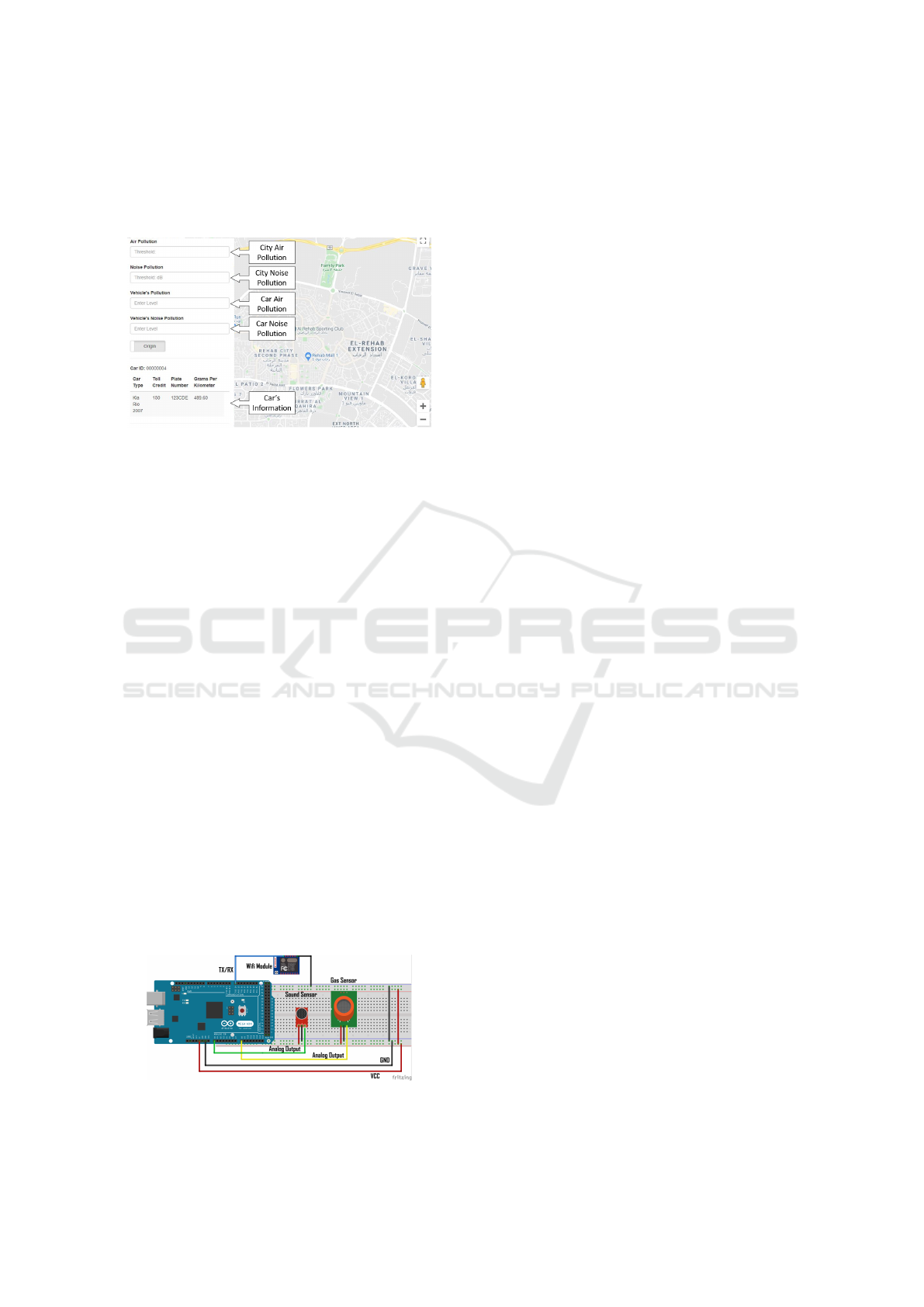
3.1.2 User Side
The second element of the system’s Software is the
user application.
Figure 4: User Application.
Through this app, the user enters the car’s UID
to be able to open a map, as shown in Figure 4, that
contains the car detailed information, including its
model, plate number, average amount of produced
emissions in Grams per Kilometer, and the current
credit. This credit represents the amount of money the
user precharged to pay future pollution related tolls or
taxes. The application also shows the car’s real-time
emission data from the embedded sensors. The ap-
plication allows the user to choose the desired origin
and destination points, so the server can generate the
routes based on the routing algorithm implemented,
see Figure 6.
3.2 Hardware Implementation
To measure in real-time pollution levels of both the
car and the city, different sensor nodes were used.
Each sensor node includes different types of sensors
connected to an Arduino board and a Node MCU. For
air pollution data, different gas sensors are used: an
MQ-7 to measure Carbon Monoxide and an MQ-135
to measure Nitrogen Oxides and Carbon Monoxide.
For noise pollution data, a sound sensor is used to
measure the decibel value of the noise pollution. The
sensor nodes, as implemented in Figure 5, are embed-
ded in the car, as well as in the city infrastructure.
Figure 5: The hardware circuit used in measuring air and
noise pollution.
3.3 Routing Algorithm
The routing algorithm proposed takes into considera-
tion the car’s origin and destination points, car’s cur-
rent pollution level, the city’s current pollution level
and the city’s pollution preset thresholds.
The system provides the user with two possible
routes: 1-the pollution optimized route, which adds
into consideration the amount of emissions and noise
the car produces, and the distance that the car will
travel inside the city. The algorithm tends to minimize
the distance travelled inside the city, if the pollution
levels are high. 2-the ’normal’ shortest path based on
Google Map’s Routing API, which takes into consid-
eration the time, distance, and traffic.
The algorithm flows as follow: the user enters the
origin and destination points, the system checks if any
of the points is inside the boundary of a defined city
on the server side. Next, it takes the real-time readings
of the pollution of the car and the concerned city. Fi-
nally, it generates the possible routes. Figure 6 shows
an overview of the routing algorithm and Algorithm 1
shows an example of exiting a city in details.
When the pollution levels are high, the algorithm
works as follows: If the destination point is inside a
defined city, in order to minimize the distance trav-
elled inside the city, it checks all the possible entry
points and calculates the distance between each one
of them and the destination point. It takes the nearest
entry point to the destination and adds it as a ”way
point”; this is from where the user should enter the
city. The route is then generated by connecting the
shortest path from the origin point to the selected en-
try point and the shortest path from the entry point
and the destination point together.
If the origin point is inside a defined city, then it
checks all the possible exit points and calculates the
distance between each of them and the origin point.
The nearest exit to the origin point becomes a ”way
point” on the route and then the full route is generated.
Lastly, if both origin and destination points are in-
side a defined city, it compares the direct route from
the origin to the destination and a route that exits the
city and re-enters it. This is done by adding the dis-
tance travelled inside the city from the origin to its
nearest exit point and from the nearest entry point to
the destination. If this exit and reenter route’s segment
is shorter inside the city than the direct path from the
origin to the destination, it would be chosen as the
pollution optimized route.
Naturally, when the pollution levels are below the
threshold, the routing algorithm generates only the di-
rect shortest path, without any concerns about the dis-
tance travelled inside the city.
An Intelligent Transportation System for Air and Noise Pollution Management in Cities
337
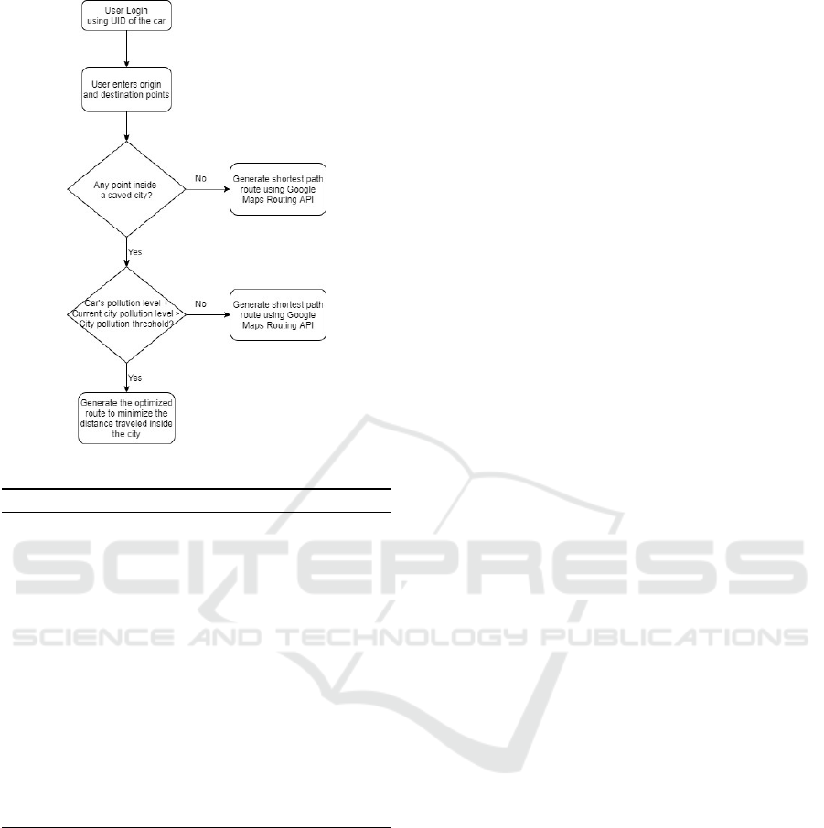
Figure 6: Overview of the ITS Routing Algorithm.
Algorithm 1: Routing Algorithm to get out of the city.
Input: Car’s ID uid, Start Point start, Destination Point dest,
Car’s Pollution Level carPoll, City’s Pollution Level cityPoll,
City’s Pollution Threshold cityT hresh
Output: Routes R1, R2
1: if (start inside city) then
2: if (carPoll + cityPoll > cityT hresh) then
3: for Gate g in cityExitGates do
4: Distance d = Distance between start and g
5: Add Gate g with the minimum d to the Route R1 Way
Points
6: end for
7: else
8: R1 = Shortest Path
9: end if
10: R2 = Shortest Path
11: end if
12: return R1 and R2
4 TESTING AND RESULTS
4.1 Testing Scenarios
To test the functionality of the system, six different
scenarios were simulated. While the first three sce-
narios allow testing the system in the case of high pol-
lution levels, the next three scenarios allow testing the
system with low pollution levels.
• Scenario 1: Origin point is not inside a defined
city, destination point is inside a defined city, and
the car’s pollution level is high enough to make
the city’s pollution level higher than the thresh-
olds (Figure 8).
• Scenario 2: Origin point is inside a defined city,
destination point is not inside a defined city, and
the city’s pollution level will exceed the thresh-
olds (Figure 9).
• Scenario 3: Origin and destination points are in-
side the city, and the car’s pollution level is high
(Figure 10).
• Scenario 4: Origin point is not inside a defined
city, destination point is inside a defined city, and
the car’s pollution level is low (Figure 11)
• Scenario 5: Origin point is inside a defined city,
destination point is not inside a defined city, and
the car’s pollution level is low (Figure 12).
• Scenario 6: Origin and destination points are in-
side a city, and the car’s pollution level is low
(Figure 13).
4.2 Results
This section presents the simulation output of the sys-
tem using the six testing scenarios.
For each scenario, in addition to the routes, mis-
cellaneous information about each route is also pro-
vided to the user. This information includes: the total
distance, total emissions, total fuel consumed, as well
as the distance travelled and emissions produced in-
side the city; e.g. figure 7.
Figures 8 to 13 show the outcome of the six different
testing scenarios.
5 CONCLUSION
Because air quality and noise levels in urban cities
have become major environmental concerns world-
wide, managing road vehicles which are considered
a primary source of air pollution and also a consid-
erable source of noise pollution in urban cities be-
comes crucial. In this paper, an IoT based Intelligent
Transportation System-ITS for Air and Noise pollu-
tion management in cities is proposed. Our ITS pro-
posed uses real-time pollution data to route cars based
on the measured particle emissions and noise levels.
Our system is divided into two layers: software and
hardware. The software layer includes two different
parts: the server side which is managed by an admin
and where cities are defined with boundaries, entry
and exit points, have air and noise pollution thresh-
olds; and the user side which informs the driver about
the pollution levels and the possible routes: city-
pollution optimized and ”normal” shortest route. Our
system aims at helping in keeping a city’s pollution
VEHITS 2021 - 7th International Conference on Vehicle Technology and Intelligent Transport Systems
338
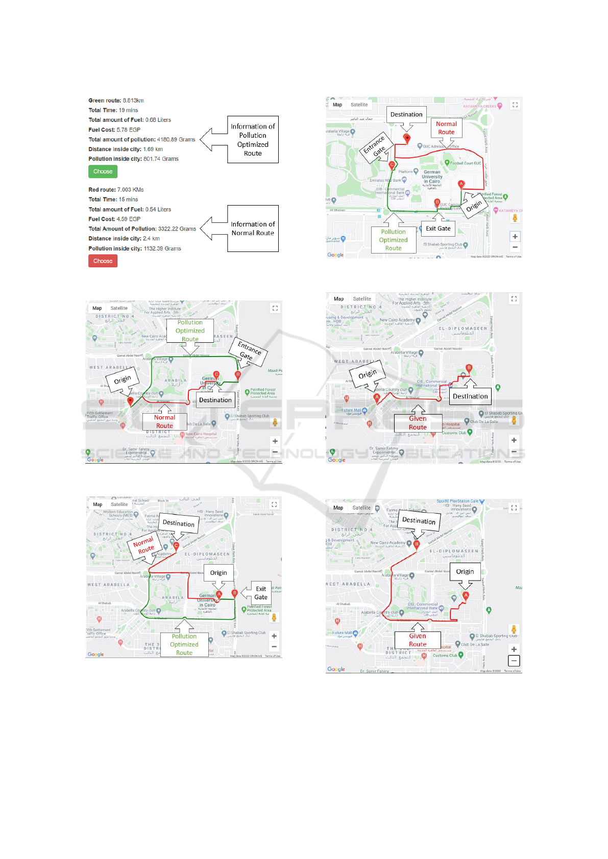
Figure 7: Information provided to the user about the routes
given by the system.
Figure 8: Scenario 1, origin point is outside the city, desti-
nation point is inside the city, with high pollution levels.
Figure 9: Scenario 2, origin point is inside the city, destina-
tion point is outside the city, with high pollution levels.
level under a predefined threshold. To verify the fea-
sibility of our approach, six different test scenarios
were simulated and their outcomes were verified for
one defined city. In the future, we plan to test our
Figure 10: Scenario 3, origin point is inside the city, desti-
nation point is inside the city, with high pollution levels.
Figure 11: Scenario 4, origin point is outside the city, desti-
nation point is inside the city, with low pollution levels.
Figure 12: Scenario 5, origin point is inside the city, desti-
nation point is outside the city, with low pollution levels.
systems on more cities having different configurations
and further validate our approach.
An Intelligent Transportation System for Air and Noise Pollution Management in Cities
339
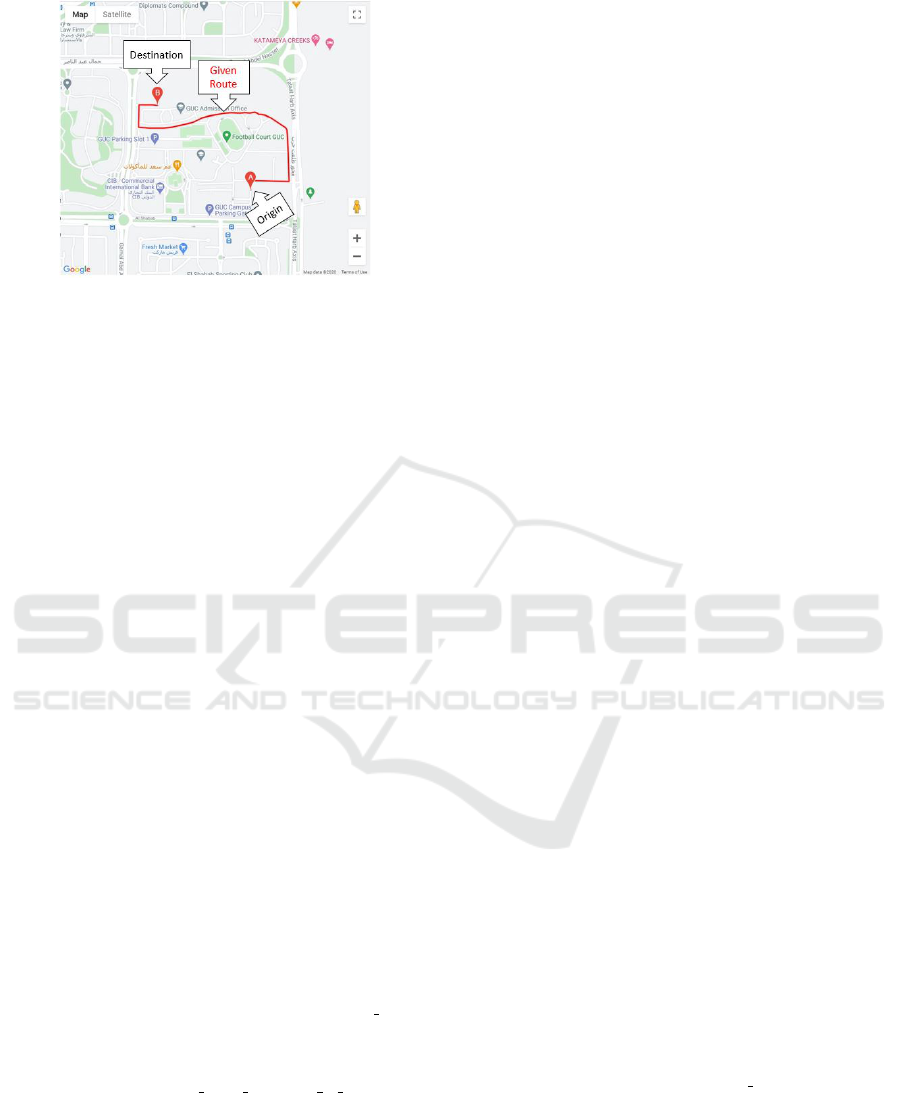
Figure 13: Scenario 6, origin point is inside the city, desti-
nation point is inside the city, with low pollution levels.
ACKNOWLEDGEMENTS
We would like to thank Omar Mokbel and Ramy
Mansour, GUC Computer Engineering students-now
graduates- for their precious contribution to the devel-
opment of the prototype used in this study.
REFERENCES
Abou-Ali, H. and Thomas, A. (2011). Regulating traffic to
reduce air pollution in greater cairo, egypt. Technical
Report 664, Economic Research Forum (ERF).
Afsharnia, M., Azizabadi, H., Poursadeghiyan, M., Hojat-
panah, R., Ghandehari, P., and Firoozi, A. (2016).
Measuring noise pollution in high-traffic streets of bir-
jand. 11:1085–1090.
Ballesteros, J. A., Sarradj, E., Fern
´
andez, M. D., Geyer, T.,
and Ballesteros, M. J. (2015). Noise source identifica-
tion with beamforming in the pass-by of a car. Applied
Acoustics, 93:106 – 119.
BBC (2020). How our daily travel harms the planet. https:
//www.bbc.com/future/article/20200317-climate-cha
nge-cut-carbon-emissions-from-your-commute.
C P, M. and Karuppanagounder, K. (2018). Economic im-
pact of traffic congestion- estimation and challenges.
European Transport - Trasporti Europei.
Canada (2019). Health impacts of air pollu-
tion in canada – estimates of morbidity out-
comes and premature mortalities - 2019 report.
http://publications.gc.ca/collections/collection 2019/
sc-hc/H144-51-2019-eng.pdf.
den Boer, E. and Schroten, A. (2007). Traffic
noise reduction in europe. https://www.cedel
ft.eu/publicatie/traffic noise reduction in europe/821.
Desarnaulds, V., Monay, G., and Carvalho, A. (2004). Noise
reduction by urban traffic management.
Dhingra, S., Madda, R., Gandomi, A., Patan, R., and
Daneshmand, M. (2019). Internet of things mobile
- air pollution monitoring system (iot-mobair). IEEE
Internet of Things Journal, PP:1–1.
EEA (2019). Road traffic remains biggest source
of noise pollution in europe. https://www.
eea.europa.eu/highlights/road-traffic-remains-big
gest-source.
EEA (2020). Noise. https://www.eea.europa.eu/soer/2015/
/noise.
Fiedler, P. E. K. and Zannin, P. H. T. (2015). Evaluation
of noise pollution in urban traffic hubs—noise maps
and measurements. Environmental Impact Assessment
Review, 51:1 – 9.
Fueleconomy.gov (2020). Fueleconomy.gov - the official
u.s. government source for fuel economy information.
Guanochanga, B., Cachipuendo, R., Fuertes, W., Salvador,
S., Benitez, D., Toulkeridis, T., Torres, J., Villac
´
ıs, C.,
Tapia Leon, F., and Meneses, F. (2019). Real-Time Air
Pollution Monitoring Systems Using Wireless Sensor
Networks Connected in a Cloud-Computing, Wrapped
up Web Services: Volume 1, pages 171–184.
IOMVM (2019). 2005-2019 sales statistics. http://www.
oica.net/category/sales-statistics/.
Jereb, B., Kumper
ˇ
s
ˇ
cak, S., and Bratina, T. (2018). The im-
pact of traffic flow on fuel consumption increase in the
urban environment. FME Transactions, 46:278–284.
Kumar, S. (2017). Cloud based vehicle pollution detection
and monitoring system.
Kundu, S. and Maulik, U. (2020). Vehicle Pollution Detec-
tion from Images Using Deep Learning, pages 1–5.
Lopez-Aparicio, S., Grythe, H., Thorne, R. J., and Vogt, M.
(2020). Costs and benefits of implementing an envi-
ronmental speed limit in a nordic city. Science of The
Total Environment, 720:137577.
Miralavy, S., Ebrahimi Atani, R., and Khoshrouz, N.
(2019). A wireless sensor network based approach to
monitor and control air pollution in large urban areas.
Muthumurugan, H. (2018). Integrated automated system
for monitoring and alerting vehicle pollution. Inter-
national Journal of Trend in Scientific Research and
Development, Volume-3:1294–1297.
Prezelj, J. and Murovec, J. (2017). Traffic noise modelling
and measurement: Inter-laboratory comparison. Ap-
plied Acoustics, 127:160–168.
Reshi, A. A., Shafi, S., and Kumaravel, A. (2013). Vehn-
ode: Wireless sensor network platform for automobile
pollution control. In 2013 IEEE Conference on Infor-
mation Communication Technologies, pages 963–966.
Retallack, A. E. and Ostendorf, B. (2020). Relationship
between traffic volume and accident frequency at in-
tersections. International Journal of Environmental
Research and Public Health, 17(4).
Subramani, T., Kavitha, M., and Sivaraj, K. (2012). Model-
ling of traffic noise pollution. Int J. Eng Res Appl,2.
USEPA (2018). Sources of greenhouse gas emissio-
ns. https://www.epa.gov/ghgemissions/sources-green
house-gas-emissions.
WHO (2011). Burden of disease from environmental noise-
quantification of healthy life years lost in europe.
https://www.who.int/quantifying ehimpacts/publicati
ons/e94888/en/.
WHO (2020). Road traffic injuries. https://www.who.
int/news-room/fact-sheets/detail/road-traffic-injuries.
Wokekoro, E. (2020). Public awareness of the impacts of
noise pollution on human health. World Journal of
Research and Review (WJRR), 10:27–32.
Worldometer (2020). Current world population. https://
www.worldometers.info/world-population/.
VEHITS 2021 - 7th International Conference on Vehicle Technology and Intelligent Transport Systems
340
