A Global Density-based Approach for Instance Selection
Joel Lu
´
ıs Carbonera
a
Institute of informatics, Federal University of Rio Grande do Sul, Porto Alegre, Brazil
Keywords:
Instance Selection, Data Reduction, Data Mining, Machine Learning, Big Data.
Abstract:
Due to the increasing size of the datasets, instance selection techniques have been applied for reducing the
computational resources involved in data mining and machine learning tasks. In this paper, we propose a
global density-based approach for selecting instances. The algorithm selects only the densest instances in
a given neighborhood and the instances in the boundaries among classes, while excludes potentially harmful
instances. Our method was evaluated on 14 well-known datasets used in a classification task. The performance
of the proposed algorithm was compared to the performances of 8 prototype selection algorithms in terms of
accuracy and reduction rate. The experimental results show that, in general, the proposed algorithm provides
a good trade-off between reduction rate and accuracy with reasonable time complexity.
1 INTRODUCTION
Prototype selection is a data-mining (or machine
learning) pre-processing task that consists of produc-
ing a smaller representative set of instances from the
total available data, which can support a data mining
task with no performance loss (or, at least, a reduced
performance loss) (Garc
´
ıa et al., 2015). Thus, every
prototype selection strategy faces a trade-off between
the reduction rate of the dataset and the resulting clas-
sification quality (accuracy) (Chou et al., 2006).
Some of the proposed algorithms for instance se-
lection, such as (Wilson and Martinez, 2000; Brighton
and Mellish, 2002) have a high time complexity,
which is an undesirable property for algorithms that
should deal with big volumes of data. Other ap-
proaches, such as (Carbonera and Abel, 2015; Car-
bonera and Abel, 2016), have a low complexity time,
but, on the other hand, produce reduced datasets that,
when used for training classifiers, cause a loss in
accuracy. In this paper, we propose a novel algo-
rithm for instance selection, called XGDIS (Extended
Global Density-based Instance Selection)
1
. The algo-
rithm selects the densest instances in a given neigh-
borhood and preserves the boundaries among differ-
ent classes, while excludes potentially harmful in-
stances.
a
https://orcid.org/0000-0002-4499-3601
1
The source code of the algorithm is available in
https://www.researchgate.net/publication/349466535
XGDIS source code
Our approach was evaluated on 14 well-known
datasets and its performance was compared with the
performance of 8 important algorithms provided by
the literature, according to 2 different performance
measures: accuracy and reduction. The accuracy
was evaluated considering two classifiers: SVM and
KNN. The results show that, when compared to the
other algorithms, XGDIS provides a good trade-off
between accuracy and reduction, while presents a rea-
sonable time complexity.
Section 2 presents some related works. Section 3
presents the notation that will be used throughout the
paper. Section 4 presents our approach. Section 5 dis-
cusses our experimental evaluation. Finally, Section 6
presents our main conclusions and final remarks.
2 RELATED WORKS
The Condensed Nearest Neighbor (CNN) algorithm
(Hart, 1968) and Reduced Nearest Neighbor algo-
rithm (RNN) (Gates, 1972) are some of the earli-
est proposals for instance selection. Both can assign
noisy instances to the final resulting set, are dependent
on the order of the instances, and have a high time
complexity. The Edited Nearest Neighbor (ENN) al-
gorithm (Wilson, 1972) removes every instance that
does not agree with the label of the majority of its k
nearest neighbors. This strategy is effective for re-
moving noisy instances, but it does not reduce the
dataset as much as other algorithms. In (Wilson and
402
Carbonera, J.
A Global Density-based Approach for Instance Selection.
DOI: 10.5220/0010402104020409
In Proceedings of the 23rd International Conference on Enterprise Information Systems (ICEIS 2021) - Volume 1, pages 402-409
ISBN: 978-989-758-509-8
Copyright
c
 2021 by SCITEPRESS – Science and Technology Publications, Lda. All rights reserved

Martinez, 2000), the authors present 5 approaches,
named the Decremental Reduction Optimization Pro-
cedure (DROP). These algorithms assume that those
instances that have x as one of their k nearest neigh-
bors are called the associates of x. Among the pro-
posed algorithms, DROP3 has the best trade-off be-
tween the reduction of the dataset and the classifi-
cation accuracy. It applies a noise-filter algorithm
such as ENN. Then, it removes an instance x if its
associates in the original training set can be correctly
classified without x. The main drawback of DROP3
is its high time complexity. The Iterative Case Fil-
tering algorithm (ICF) (Brighton and Mellish, 2002)
is based on the notions of Coverage set and Reach-
able set. The coverage set of an instance x is the
set of instances in T whose distance from x is less
than the distance between x and its nearest enemy
(instance with a different class). The Reachable set
of an instance x, on the other hand, is the set of in-
stances in T that have x in their respective coverage
sets. In this method, a given instance x is removed
from S if |Reachable(x)| > |Coverage(x)|. This algo-
rithm also has a high running time. In (Leyva et al.,
2015), the authors adopted the notion of local sets for
designing complementary methods for instance selec-
tion. In this context, the local set of a given instance
x is the set of instances contained in the largest hy-
persphere centered on x such that it does not contain
instances from any other class. The first algorithm,
called Local Set-based Smoother (LSSm), uses two
notions for guiding the process: usefulness and harm-
fulness. The usefulness u(x) of a given instance x is
the number of instances having x among the mem-
bers of their local sets, and the harmfulness h(x) is
the number of instances having x as the nearest en-
emy. For each instance x in T , the algorithm includes
x in S if u(x) ≥ h(x). Since the goal of LSSm is to
remove harmful instances, its reduction rate is lower
than most of the instance selection algorithms. The
author also proposed the Local Set Border selector
(LSBo). Firstly, it uses LSSm to remove noise, and
then, it computes the local set of every instance ∈ T .
Then, the instances in T are sorted in the ascending
order of the cardinality of their local sets. In the last
step, LSBo verifies, for each instance x ∈ T if any
member of its local set is contained in S, thus ensur-
ing the proper classification of x. If that is not the
case, x is included in S to ensure its correct classifi-
cation. The time complexity of the two approaches
is O(|T |
2
). In (Carbonera and Olszewska, 2019) the
authors propose an improvement of the LSBo algo-
rithm. In (Carbonera, 2017; Carbonera and Abel,
2018b; Carbonera and Abel, 2018c; Carbonera and
Abel, 2018a) the authors propose a set of algorithms
for instance and prototype selection that apply the no-
tion of spatial partition for finding representative data
in an efficient way. In (Carbonera and Abel, 2020b)
the authors propose an algorithm that identify clus-
ters of instances distributed around centroids identi-
fied through kernel density estimation.
In (Carbonera and Abel, 2015), the authors pro-
posed the Local Density-based Instance Selection
(LDIS) algorithm. This algorithm selects the in-
stances with the highest density in their neighbor-
hoods. It provides a good balance between accuracy
and reduction and is faster than the other algorithms
discussed here. The literature provides some exten-
sions to the basic LDIS algorithm, such as (Carbon-
era and Abel, 2016; Carbonera and Abel, 2017; Car-
bonera and Abel, 2020a). In (Malhat et al., 2020)
the authors state that LDIS is biased towards in-
creasing the reduction at the cost of accuracy and,
due to this, they propose two algorithms inspired by
LDIS algorithm for reducing this bias and increas-
ing the accuracy: global density-based instance se-
lection (GDIS) and enhanced global density-based in-
stance selection (EGDIS). Both algorithms evaluate
the density and the neighborhood of each instance in a
global perspective (instead of doing it locally, as LDIS
does), selects the densest points in their neighbor-
hood and preserve instances at the boundaries among
classes. This ensures accuracy rates that surpass those
achieved by LDIS, although the resulting algorithms
have a higher time complexity, when compared with
LDIS. In this work we propose a novel algorithm in-
spired in GDIS algorithm called XGDIS.
3 NOTATIONS
In this section, we introduce a notation adapted from
(Carbonera and Abel, 2015) that will be used through-
out the paper.
• T = {o
1
,o
2
,...,o
n
} is the non-empty set of n in-
stances (or data objects), representing the original
dataset to be reduced in the prototype selection
process.
• D = {d
1
,d
2
,...,d
m
} is a set of m dimensions (that
represent features or attributes), where each d
i
⊆
R.
• Each o
i
∈ T is an m − tuple, such that o
i
=
(o
i1
,o
i2
,..., o
im
), where o
ij
represents the value of
the j-th feature (or dimension) of the instance o
i
,
for 1 ≤ j ≤ m.
• val : T × D → R is a function that maps a data
object o
i
∈ T and a dimension d
j
∈ D to the value
A Global Density-based Approach for Instance Selection
403

o
ij
, which represents the value in the dimension d
j
for the object o
i
.
• L = {l
1
,l
2
,..., l
p
} is the set of p class labels that
are used for classifying the instances in T , where
each l
i
∈ L represents a given class label.
• l : T → L is a function that maps a given instance
x
i
∈ T to its corresponding class label l
j
∈ L.
• c : L → 2
T
is a function that maps a given class
label l
j
∈ L to a given set C, such that C ⊆ T , which
represents the set of instances in T whose class is
l
j
. Notice that T =
S
l∈L
c(l). In this notation, 2
T
represents the powerset of T , that is, the set of all
subsets of T , including the empty set and T itself.
• nn : T × R → 2
T
is a function that maps a given
object o
i
∈ T and a value k ∈ R to the k nearest
neighbors of o
i
in T , according to a given distance
function d.
• d : T × T → R is a distance function (or dissim-
ilarity function), which maps two instances to a
real number that represents the distance (or dis-
similarity) between them. This function can be
domain-dependent.
4 THE XGDIS ALGORITHM
In this paper, we propose the XGDIS (Extended
Global Density Instance Selection) algorithm, which
was inspired by the GDIS algorithm (Malhat et al.,
2020).
As the GDIS algorithm, the XGDIS algorithm
also assumes that the density of a given object can be
used for estimating the amount of information that it
represents and, therefore, its importance for support-
ing the classification of novel instances. The XGDIS
algorithm, following the approach of the GDIS algo-
rithm, adopts a global version of the density measure
adopted in the LDIS algorithm, which adopts a lo-
cal density measure. In this context, a global density
measure evaluates the density of a given object o
i
by
considering its average distance from each other ob-
ject in the whole dataset T , while the local density of
o
i
considers only its average distance from each ob-
ject whose class label is l(o
i
). Thus, the density func-
tion of a given object o
i
, denoted by dens(o
i
) is given
by:
dens(o
i
) = −
1
|T | − 1
∑
y∈T,y6=o
i
d(y,o
i
) (1)
Besides that, the XGDIS algorithm also adopts the
notion of relevance of a given instance, which was
adopted in GDIS.
Definition 1. The relevance of a given object o
i
∈
T , denoted by rel(ob jecto
i
) is the number of objects
within the k nearest neighbors of o
i
that have the same
class label of o
i
. That is:
rel(o
i
) = |{x|x ∈ nn(o
i
,k) ∧ l(o
i
) = l(x)}| (2)
The main difference regarding the XGDIS and GDIS
is that XGDIS includes an additional step for remov-
ing potentially harmful (noisy) instances. In order
to identify potentially harmful, the XGDIS algorithm
adopts the notions of usefulness and harmfulness:
Definition 2. The usefulness of an object o
i
∈ T , de-
noted by u(o
i
) measures the degree to which o
i
can
support the classification of a novel object. It is given
by the number of objects in T that have o
i
among its k
nearest neighbors and that have the same label l
i
∈ L
of o
i
. That is:
u(o
i
) = |{x|o
i
∈ nn(x, k) ∧ l(o
i
) = l(x)}| (3)
Definition 3. The harmfulness of an object o
i
∈ T ,
denoted by h(o
i
) measures the degree to which o
i
can
hinder the classification of a novel object. It is given
by the number of objects in T that have o
i
among its
k nearest neighbors and that have a label l
j
∈ L that is
different from the label of o
i
. That is:
h(o
i
) = |{x|o
i
∈ nn(x, k) ∧ l(o
i
) 6= l(x)}| (4)
By considering the previously mentioned notions, it is
possible to describe the XGDIS algorithm. It takes as
input a set of data objects T and a value k ∈ R, which
determines the size of the neighborhood of each in-
stance that the algorithm will consider. The algorithm
starts by considering S as an empty set. After that, the
algorithm evaluates each objet o
i
∈ T . And:
• If the relevance of o
i
is equal to k, this suggests
that o
i
is probably an internal object; that is, an
object that does not lie in the boundary of two
different classes. Thus, the algorithm verifies if o
i
has the highest density among its k nearest neigh-
bors. In this case, the algorithm includes o
i
in S.
• If the relevance of o
i
is greater than k/2, this sug-
gests that o
i
is probably a border object; that is,
an object that lies in the boundaries of two dif-
ferent classes. And, since its class label agrees
with the class label of the majority of its neigh-
bors, this suggests that it is not a noisy instance.
In this case, the algorithm verifies if the usefulness
of o
i
is greater or equal to its harmfulness. In this
case, this suggests that o
i
is useful for supporting
the classification of novel instances. If this is true,
the algorithm includes o
i
in S.
ICEIS 2021 - 23rd International Conference on Enterprise Information Systems
404

Algorithm 1: XGDIS algorithm.
Input: A set instances T , a value k of
neighbors.
Output: A set S of selected instances.
begin
S ←
/
0;
foreach o
i
∈ T do
if rel(o
i
) = k then
f oundDenser ←false;
foreach n
j
∈ nn(o
i
,k) do
if dens(o
i
) < dens(n
j
) then
f oundDenser ← true;
if ¬ f oundDenser then
S ← S ∪ {o
i
};
else if rel(o
i
) ≥
k
2
then
if u(o
i
) ≥ h(o
i
) then
S ← S ∪ {o
i
};
return S;
Since the algorithm needs to compare each object in
T with each other object in T in order to calculate the
density of each object, the overall time complexity of
XGDIS is proportional to O(|T |
2
).
5 EXPERIMENTS
For evaluating our approach, we compared the
XGDIS algorithm in a classification task, with 8 im-
portant prototype selection algorithms
2
provided by
the literature: DROP3, ENN, ICF, LSBo, LSSm,
LDIS, GDIS and EGDIS. We considered 14 well-
known datasets with numerical dimensions: car-
diotocography, diabetes, E. Coli, glass, heart-statlog,
ionosphere, iris, landsat, letter, optdigits, page-
blocks, parkinson, segment, spambase and wine. All
datasets were obtained from the UCI Machine Learn-
ing Repository
3
.
We use two standard measures to evaluate the per-
formance of the algorithms: accuracy and reduction.
Following (Leyva et al., 2015; Carbonera and Abel,
2015), we assume: accuracy = |Sucess(Test)|/|Test|
and reduction = (|T |− |S|)/|T |, where Test is a given
set of instances that are selected for being tested in a
classification task, and |Success(Test)| is the number
of instances in Test correctly classified in the classifi-
cation task.
For evaluating the classification accuracy of new
instances in each respective dataset, we adopted a
SVM and a KNN classifier. For the KNN classifier,
2
All algorithms were implemented by the authors.
3
http://archive.ics.uci.edu/ml/
we considered k = 3, as assumed in (Leyva et al.,
2015; Carbonera and Abel, 2015). For the SVM,
following (Anwar et al., 2015), we adopted the im-
plementation provided by Weka 3.8, with the stan-
dard parametrization ( c = 1.0, toleranceParameter =
0.001, epsilon = 1.0E − 12, using a polynomial ker-
nel and a multinomial logistic regression model with
a ridge estimator as calibrator).
Besides that, following (Carbonera and Abel,
2015), the accuracy and reduction were evaluated
in an n-fold cross-validation scheme, where n = 10.
Thus, firstly a dataset is randomly partitioned in 10
equally sized subsamples. From these subsamples, a
single subsample is selected as validation data (Test),
and the union of the remaining 9 subsamples is con-
sidered the initial training set (IT S). Next, a pro-
totype selection algorithm is applied for reducing
the IT S, producing the reduced training set (RT S).
At this point, we can measure the reduction of the
dataset. Finally, the RT S is used as the training set
for the classifier, which is used for classifying the in-
stances in Test. At this point, we can measure the
accuracy achieved by the classifier, using RT S as the
training set. This process is repeated 10 times, with
each subsample used once as Test. The 10 values
of accuracy and reduction are averaged to produce,
respectively, the average accuracy (AA) and average
reduction (AR). Notice that we have used the same
folds for all algorithms. Tables 1, 2 and 3 report, re-
spectively, for each combination of dataset and pro-
totype selection algorithm: the resulting AA achieved
by the SVM classifier, AA achieved by the KNN clas-
sifier, and the AR. The best results for each dataset is
marked in bold typeface.
In all experiments, we adopted k = 3 for DROP3,
ENN, ICF, LDIS, GDIS, EGDIS and XGDIS. Besides
that, for the algorithms that use distance (dissimilar-
ity) function, we adopted the following distance func-
tion (Carbonera and Abel, 2015):
d(x,y) =
m
∑
j=1
θ
j
(x,y) (5)
where
θ
j
(x,y) =
(
α(x
j
,y
j
), if j is a categorical feature
|x
j
− y
j
|, if j is a numerical feature
(6)
where
α(x
j
,y
j
) =
(
1, if x
j
6= y
j
0, if x
yj
= y
j
(7)
Tables 1 and 2 show that LSSm achieves the highest
accuracy in most of the datasets, for both classifiers.
A Global Density-based Approach for Instance Selection
405

Table 1: Comparison of the accuracy achieved by the training set produced by each algorithm, for each dataset, adopting a
SVM classifier.
Algorithm DROP3 ENN ICF LSBO LSSM LDIS GDIS EGDIS XGDIS Average
Cardiotocography 0.65 0.67 0.64 0.61 0.67 0.62 0.64 0.65 0.65 0.64
Diabetes 0.76 0.76 0.76 0.75 0.76 0.73 0.76 0.75 0.76 0.76
E.Coli 0.81 0.82 0.79 0.75 0.82 0.80 0.77 0.80 0.82 0.80
Glass 0.51 0.52 0.48 0.49 0.52 0.50 0.53 0.50 0.50 0.51
Heart-statlog 0.81 0.84 0.80 0.83 0.83 0.77 0.84 0.82 0.83 0.82
Ionosphere 0.80 0.88 0.77 0.54 0.88 0.80 0.85 0.77 0.85 0.79
Iris 0.93 0.95 0.69 0.44 0.95 0.82 0.71 0.69 0.73 0.77
Landsat 0.86 0.87 0.86 0.85 0.87 0.84 0.86 0.86 0.85 0.86
Optdigits 0.98 0.99 0.97 0.98 0.98 0.96 0.98 0.98 0.97 0.98
Page-blocks 0.93 0.94 0.93 0.92 0.94 0.93 0.94 0.93 0.93 0.93
Parkinsons 0.84 0.86 0.85 0.83 0.86 0.82 0.79 0.81 0.84 0.83
Segment 0.92 0.93 0.90 0.81 0.91 0.89 0.92 0.92 0.92 0.90
Spambase 0.90 0.89 0.90 0.89 0.90 0.88 0.91 0.91 0.91 0.90
Wine 0.95 0.95 0.93 0.95 0.96 0.94 0.95 0.95 0.95 0.95
Average 0.83 0.85 0.80 0.76 0.85 0.81 0.82 0.81 0.82 0.82
Table 2: Comparison of the accuracy achieved by the training set produced by each algorithm, for each dataset, adopting a
KNN classifier.
Algorithm DROP3 ENN ICF LSBO LSSM LDIS GDIS EGDIS XGDIS Average
Cardiotocography 0.61 0.66 0.60 0.56 0.68 0.54 0.61 0.61 0.61 0.61
Diabetes 0.73 0.73 0.71 0.69 0.73 0.69 0.69 0.65 0.72 0.70
E.Coli 0.84 0.85 0.82 0.78 0.85 0.84 0.80 0.76 0.82 0.82
Glass 0.62 0.64 0.61 0.54 0.68 0.61 0.63 0.65 0.63 0.62
Heart-statlog 0.69 0.70 0.67 0.66 0.68 0.68 0.69 0.60 0.68 0.67
Ionosphere 0.86 0.89 0.87 0.89 0.91 0.84 0.89 0.89 0.90 0.88
Iris 0.97 0.97 0.95 0.92 0.96 0.95 0.95 0.92 0.95 0.95
Landsat 0.89 0.90 0.86 0.86 0.90 0.87 0.88 0.88 0.88 0.88
Optdigits 0.97 0.98 0.91 0.91 0.98 0.93 0.95 0.95 0.95 0.95
Page-blocks 0.95 0.96 0.95 0.94 0.96 0.94 0.95 0.94 0.95 0.95
Parkinsons 0.84 0.86 0.80 0.83 0.86 0.81 0.83 0.83 0.83 0.83
Segment 0.94 0.95 0.91 0.87 0.95 0.90 0.93 0.93 0.93 0.92
Spambase 0.82 0.84 0.83 0.84 0.85 0.76 0.83 0.83 0.83 0.83
Wine 0.72 0.72 0.72 0.78 0.77 0.70 0.80 0.82 0.77 0.76
Average 0.82 0.83 0.80 0.79 0.84 0.79 0.82 0.80 0.82 0.81
Table 3: Comparison of the reduction achieved by each algorithm, for each dataset.
Algorithm DROP3 ENN ICF LSBO LSSM LDIS GDIS EGDIS XGDIS Average
Cardiotocography 0.70 0.31 0.71 0.70 0.13 0.86 0.49 0.38 0.62 0.54
Diabetes 0.77 0.31 0.86 0.76 0.13 0.91 0.46 0.37 0.59 0.57
E.Coli 0.71 0.16 0.87 0.82 0.09 0.90 0.64 0.57 0.71 0.61
Glass 0.75 0.32 0.68 0.72 0.14 0.90 0.52 0.41 0.66 0.57
Heart-statlog 0.73 0.30 0.79 0.68 0.14 0.92 0.42 0.31 0.56 0.54
Ionosphere 0.80 0.11 0.92 0.86 0.04 0.90 0.80 0.74 0.82 0.67
Iris 0.71 0.04 0.59 0.93 0.06 0.89 0.82 0.79 0.83 0.63
Landsat 0.72 0.10 0.90 0.88 0.05 0.92 0.70 0.67 0.74 0.63
Optdigits 0.71 0.02 0.92 0.90 0.02 0.91 0.82 0.81 0.82 0.66
Page-blocks 0.71 0.04 0.95 0.96 0.03 0.86 0.81 0.79 0.82 0.67
Parkinsons 0.70 0.15 0.75 0.86 0.11 0.81 0.56 0.54 0.65 0.57
Segment 0.69 0.04 0.83 0.91 0.04 0.83 0.75 0.74 0.76 0.62
Spambase 0.74 0.16 0.81 0.81 0.08 0.83 0.57 0.52 0.63 0.57
Wine 0.72 0.23 0.77 0.78 0.10 0.87 0.52 0.46 0.62 0.56
Average 0.73 0.16 0.81 0.83 0.08 0.88 0.63 0.58 0.70 0.60
This is expected, since that LSSm was designed for
removing noisy instances and does not provide high
reduction rates. Besides that, for most of the datasets,
the difference between the accuracy of XGDIS and
the accuracy achieved by the LSSm is not big. The
average accuracy achieved by XGDIS is similar to
the average accuracy of LSSm. It is important to no-
tice also that XGDIS has an accuracy rate that is sim-
ilar to the accuracy achieved by GDIS and EGDIS.
In cases where the achieved accuracy is lower than
the accuracy provided by other algorithms, this can
be compensated by a higher reduction produced by
XGDIS. Table 3 shows that LDIS achieves the high-
est reduction in most of the datasets, and achieves also
ICEIS 2021 - 23rd International Conference on Enterprise Information Systems
406

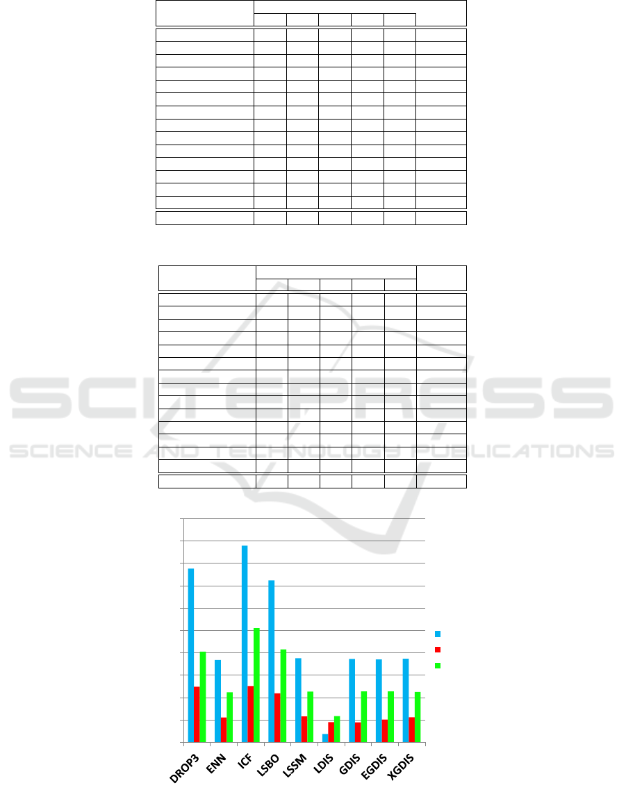
Table 4: The accuracy of a SVM classifier trained with the instances selected by the XGDIS algorithm, in different datasets,
with different values of the parameter k.
Algorithm
Value of k
Average
2 3 5 10 20
Cardiotocography 0.65 0.65 0.66 0.66 0.63 0.65
Diabetes 0.75 0.76 0.76 0.76 0.76 0.76
E.Coli 0.84 0.82 0.82 0.82 0.82 0.82
Glass 0.47 0.50 0.46 0.48 0.50 0.48
Heart-statlog 0.82 0.83 0.84 0.84 0.84 0.83
Ionosphere 0.83 0.85 0.78 0.80 0.86 0.82
Iris 0.81 0.73 0.69 0.70 0.65 0.71
Landsat 0.86 0.85 0.86 0.85 0.86 0.86
Optdigits 0.98 0.97 0.97 0.97 0.98 0.98
Page-blocks 0.94 0.93 0.93 0.94 0.94 0.94
Parkinsons 0.82 0.84 0.84 0.86 0.83 0.84
Segment 0.92 0.92 0.89 0.77 0.92 0.88
Spambase 0.90 0.91 0.90 0.90 0.90 0.90
Wine 0.95 0.95 0.95 0.95 0.94 0.95
Average 0.82 0.82 0.81 0.81 0.82 0.82
Table 5: The reduction rate achieved by the XGDIS algorithm, in different datasets, with different values of the parameter k.
Algorithm
Value of k
Average
2 3 5 10 20
Cardiotocography 0.64 0.62 0.59 0.57 0.58 0.60
Diabetes 0.65 0.59 0.52 0.41 0.33 0.50
E.Coli 0.72 0.71 0.66 0.57 0.43 0.62
Glass 0.71 0.66 0.65 0.67 0.54 0.65
Heart-statlog 0.67 0.56 0.46 0.36 0.33 0.48
Ionosphere 0.80 0.82 0.81 0.77 0.64 0.77
Iris 0.75 0.83 0.85 0.79 0.63 0.77
Landsat 0.70 0.74 0.78 0.77 0.71 0.74
Optdigits 0.75 0.82 0.88 0.87 0.79 0.82
Page-blocks 0.74 0.82 0.89 0.90 0.87 0.84
Parkinsons 0.61 0.65 0.66 0.57 0.34 0.57
Segment 0.67 0.76 0.83 0.83 0.74 0.76
Spambase 0.65 0.63 0.58 0.45 0.34 0.53
Wine 0.66 0.62 0.63 0.65 0.55 0.62
Average 0.69 0.70 0.70 0.66 0.56 0.66
0
10000
20000
30000
40000
50000
60000
70000
80000
90000
100000
optdigits
page-blocks
spambase
Milliseconds
Figure 1: Comparison of the running times of 9 prototype selection algorithms, considering the three biggest datasets. Notice
that the time axis uses a logarithmic scale.
A Global Density-based Approach for Instance Selection
407

the highest average reduction rate. However, on the
other hand, LDIS has a lower accuracy when com-
pared with XGDIS. Regarding the reduction rate, no-
tice also that XGDIS achieves higher scores in com-
parison with GDIS and EGDIS, which were used for
inspiring the strategy adopted by XGDIS.
We also carried out experiments for evaluating
the impact of the parameter k in the performance of
XGDIS. The Table 4 represents the accuracy achieved
by the SVM classifier (with the standard parametriza-
tion of Weka 3.8) trained with the instances selected
by XGDIS algorithm in different datasets, while Table
5 represents the reduction rate achieved by XGDIS al-
gorithm in each dataset. In this experiment, we con-
sidered k assuming the values 2, 5, 10, 20. We also
considered the 10-fold cross validation schema in this
experiment.
Tables 4 and 5 suggest that the behavior of XGDIS
algorithm is not so sensitive to changes in the param-
eter k, since the values of accuracy and reduction are
very similar with different values of k. Besides that,
there is no clear pattern regarding the relationship be-
tween the parameter k and the accuracy and reduction.
This suggests that there is a complex interaction be-
tween the parameter k and the intrinsic properties of
each dataset.
We also carried out a comparison of the running
times of the prototype selection algorithms consid-
ered in our experiments. In this comparison, we ap-
plied the 9 prototype selection algorithms to reduce
the 3 biggest datasets considered in our tests: page-
blocks, optdigits and spambase. We adopted the same
parametrizations that were adopted in the first exper-
iment. We performed the experiments in an Intel
R

Core
TM
i5-5200U laptop with a 2.2 GHz CPU and
8 GB of RAM. The Figure 1 shows that, considering
these datasets, the LDIS algorithm has the lowest run-
ning times in all datasets. However, it is importante
to notice that GDIS, EGDIS and XGDIS algorithms
have reasonable running times when compared with
the other algorithms. And, besides that, these three
algorithms have a very similar running time.
In summary, the experiments show that XGDIS
presents a good balance between reduction rate, accu-
racy and running time. Besides that, the running time
of XGDIS is lower than the running time of classic al-
gorithms such as DROP3 and ICF, but is higher than
the running time of LDIS. However, it is important
to notice that XGDIS has the higher accuracy in most
of the datasets in comparison with LDIS. We com-
pared with GDIS and EGDIS, the XGDIS algorithm
achieved a similar accuracy and, higher reduction rate
and a similar running time. Thus, this suggests that
XGDIS can be viewed as an improvement over GDIS
and EGDIS.
6 CONCLUSION
In this paper, we proposed an algorithm for instance
selection, called XGDIS. It uses the notion of den-
sity for identifying instances that can represent a high
amount of information of the dataset. In summary,
the algorithm selects the instances whose density is
higher than the density of their neighbors, while re-
move instances that can be harmful for the classifica-
tion of novel instances.
The experiments show that XGDIS presents a
good balance between reduction rate, accuracy and
running time. Besides that, the algorithm can be
viewed as an improvement over the GDIS and EGDIS
algorithms, which were considered as a basis for the
development of XGDIS.
In future works, we plan to investigate how to im-
prove the performance of the XGDIS algorithm.
REFERENCES
Anwar, I. M., Salama, K. M., and Abdelbar, A. M. (2015).
Instance selection with ant colony optimization. Pro-
cedia Computer Science, 53:248–256.
Brighton, H. and Mellish, C. (2002). Advances in instance
selection for instance-based learning algorithms. Data
mining and knowledge discovery, 6(2):153–172.
Carbonera, J. L. (2017). An efficient approach for instance
selection. In International Conference on Big Data
Analytics and Knowledge Discovery, pages 228–243.
Springer.
Carbonera, J. L. and Abel, M. (2015). A density-based
approach for instance selection. In Tools with Arti-
ficial Intelligence (ICTAI), 2015 IEEE 27th Interna-
tional Conference on, pages 768–774. IEEE.
Carbonera, J. L. and Abel, M. (2016). A novel density-
based approach for instance selection. In 2016 IEEE
28th International Conference on Tools with Artificial
Intelligence (ICTAI), pages 549–556. IEEE.
Carbonera, J. L. and Abel, M. (2017). Efficient prototype
selection supported by subspace partitions. In 2017
IEEE 29th International Conference on Tools with Ar-
tificial Intelligence (ICTAI), pages 921–928. IEEE.
Carbonera, J. L. and Abel, M. (2018a). Efficient instance
selection based on spatial abstraction. In 2018 IEEE
30th international conference on tools with artificial
intelligence (ICTAI), pages 286–292. IEEE.
Carbonera, J. L. and Abel, M. (2018b). An efficient proto-
type selection algorithm based on dense spatial parti-
tions. In International Conference on Artificial Intelli-
gence and Soft Computing, pages 288–300. Springer.
Carbonera, J. L. and Abel, M. (2018c). An efficient proto-
type selection algorithm based on spatial abstraction.
ICEIS 2021 - 23rd International Conference on Enterprise Information Systems
408

In International Conference on Big Data Analytics
and Knowledge Discovery, pages 177–192. Springer.
Carbonera, J. L. and Abel, M. (2020a). An attraction-based
approach for instance selection. In 2020 IEEE 32nd
International Conference on Tools with Artificial In-
telligence (ICTAI), pages 1053–1058. IEEE.
Carbonera, J. L. and Abel, M. (2020b). A density-based
prototype selection approach. In International Con-
ference on Artificial Intelligence and Soft Computing,
pages 117–129. Springer.
Carbonera, J. L. and Olszewska, J. I. (2019). Local-set
based-on instance selection approach for autonomous
object modelling. International Journal of Advanced
Computer Science and Applications, 10(12):Paper–1.
Chou, C.-H., Kuo, B.-H., and Chang, F. (2006). The gen-
eralized condensed nearest neighbor rule as a data re-
duction method. In Pattern Recognition, 2006. ICPR
2006. 18th International Conference on, volume 2,
pages 556–559. IEEE.
Garc
´
ıa, S., Luengo, J., and Herrera, F. (2015). Data prepro-
cessing in data mining. Springer.
Gates, G. W. (1972). Reduced nearest neighbor rule. IEEE
Transactions on Information Theory, 18(3):431–433.
Hart, P. E. (1968). The condensed nearest neighbor rule.
IEEE Transactions on Information Theory, 14:515–
516.
Leyva, E., Gonz
´
alez, A., and P
´
erez, R. (2015). Three
new instance selection methods based on local sets:
A comparative study with several approaches from
a bi-objective perspective. Pattern Recognition,
48(4):1523–1537.
Malhat, M., El Menshawy, M., Mousa, H., and El Sisi, A.
(2020). A new approach for instance selection: Algo-
rithms, evaluation, and comparisons. Expert Systems
with Applications, 149:113297.
Wilson, D. L. (1972). Asymptotic properties of nearest
neighbor rules using edited data. IEEE Transactions
on Systems, Man and Cybernetics, SMC-2(3):408–
421.
Wilson, D. R. and Martinez, T. R. (2000). Reduction tech-
niques for instance-based learning algorithms. Ma-
chine learning, 38(3):257–286.
A Global Density-based Approach for Instance Selection
409