LPO Proofs in Two Educational Contexts
Engelbert Hubbers
a
Institute for Computing and Information Sciences, Radboud University, Nijmegen, The Netherlands
Keywords:
Term Rewriting Systems, Lexicographical Path Order, Tree Style Proof, Fitch Style Proof, Digital Exams.
Abstract:
The purpose of this paper is twofold. First, it introduces several styles for constructing and writing down
mathematical proofs for a specific technique used in theoretical Computing Science. Second, an inventory
of pros and cons of these proof styles is made in two educational contexts, namely whether the proof styles
help students in understanding the proofs, and whether the proof styles are practical in both written and digital
exams. It turns out that there is no clear winner in both contexts, but the newly introduced so-called shuffled
Fitch style is the most practical choice.
1 INTRODUCTION
For several years the author has been involved in
teaching an introductory course on Term Rewriting
Systems (TRS) and λ-calculus to second-year Com-
puting Science students. With respect to the TRS
part, basically three topics are discussed: reduction,
termination, and confluence. For the termination
part, two proof methods are introduced: the seman-
tical method of polynomial monotonic interpretations
(Terese, 2003), and the syntactical method of lexico-
graphic path order, or LPO in short, (Kamin and Levy,
1980; Dershowitz, 1982; Terese, 2003).
After introducing these methods and having the
students do a homework assignment about this topic,
the author always asks which method is preferred
by the students. And typically, they vote like 90%
in favor of the polynomial monotonic interpretations.
Even though they know that one of the benefits of the
LPO method is that they can build the requested order
on the fly: even if students don’t have a clue about a
useful order, they can simply start applying the rules
and then derive such an order. At the exam, often the
TRS to be studied is chosen in such a way that both
techniques can be used for proving termination of the
system. And again, most students opt for the polyno-
mial monotonic interpretations. For instance, in the
exam of 2020, 34 out of 42 students chose the method
of polynomial monotonic interpretations. However,
every now and then there is an exam where students
are enforced to apply the LPO method, and this usu-
ally leads to bad results. Students seem to get lost in
a
https://orcid.org/0000-0002-6182-6493
all the nested applications of the definition of >
lpo
as
given below in Definition 1.
In order to solve this problem a few different styles
of visualizations of such an LPO proof are presented
in this paper. After describing some benefits and
drawbacks with respect to the educational objective of
letting the students understand the proofs better, it is
also discussed whether these proof styles can be used
easily in both written and digital exams.
Because this paper is not about comparing the
two different methods for proving termination, but
specifically about improving the didactics for the LPO
method, we do not explain the details for the polyno-
mial monotonic interpretations method.
2 THE LPO THEORY
The method of LPO was introduced in (Kamin and
Levy, 1980). Later on, many slightly different vari-
ants have been published, for instance in (Dershowitz,
1982; Baader and Nipkow, 1998; Terese, 2003). Ac-
tually, some of these versions are considered more
practical than Definition 1 below, however, this pa-
per is about the author’s course which happens to use
course notes (Zantema, 2014) with the following def-
inition:
Definition 1 (>
lpo
). Let > be an order on the set of
function symbols. Let f and g be function symbols.
And let t
1
, . . . , t
n
, u, u
1
, . . . , u
m
be terms. Then
f (t
1
,...,t
n
)>
lpo
u if and only if
1. there exists i ∈ {1,...,n} such that
270
Hubbers, E.
LPO Proofs in Two Educational Contexts.
DOI: 10.5220/0010399402700278
In Proceedings of the 13th International Conference on Computer Supported Education (CSEDU 2021) - Volume 1, pages 270-278
ISBN: 978-989-758-502-9
Copyright
c
 2021 by SCITEPRESS – Science and Technology Publications, Lda. All rights reserved

(a) t
i
= u, or
(b) t
i
>
lpo
u
or
2. u = g(u
1
,...,u
m
) and for all i ∈ {1, . . . , m} it holds
that f (t
1
,...,t
n
)>
lpo
u
i
and either
(a) f > g, or
(b) f = g and (t
1
,...,t
n
) >
lex
lpo
(u
1
,...,u
m
).
Rule 2b refers to >
lex
lpo
, which is defined as follows:
Definition 2 (>
lex
lpo
). Let t
1
, . . . , t
n
, u
1
, . . . , u
m
be
terms. Then (t
1
,...,t
n
) >
lex
lpo
(u
1
,...,u
m
) if and only
if
1. n = m, and
2. there exists i ∈ {1,...,n} such that
(a) t
i
>
lpo
u
i
and
(b) for all j ∈ {1, . . . , i − 1} it holds that t
j
= u
j
.
And this is the main theorem behind the LPO method:
Theorem 3. Let R be a TRS. If ` >
lpo
r for all ` → r
in R, then R is terminating.
So in order to prove that ` >
lpo
r for some ` → r
in R, students have to apply Rules 1b, 2a and 2b re-
peatedly until they end up with a proof obligation
for which they can apply one of the closing rules,
Rules 1a, 2a and 2b.
As a running example in this paper, we will apply
the technique on the two-parameter version of the so-
called Ackermann function (Ackermann, 1928; P
´
eter,
1935; Robinson, 1948):
Example 4. Consider the TRS R defined by these
rules:
A(0,n) → s(n)
A(s(m),0) → A(m,s(0))
A(s(m),s(n)) → A(m,A(s(m),n))
Show that R is terminating by using the lexicographic
path order given that A > s > 0. Because of Theo-
rem 3 we know that it suffices to show that:
1. A(0,n)>
lpo
s(n)
2. A(s(m),0)>
lpo
A(m,s(0))
3. A(s(m),s(n))>
lpo
A(m,A(s(m),n))
3 PROOF STYLES
We now continue by presenting proofs of termination
of the TRS R from Example 4 using different styles.
3.1 Natural Language Style Proofs
In the literature, LPO proofs are usually given in
the form of natural languages proofs, for instance in
the classic works (Baader and Nipkow, 1998) and
(Terese, 2003). Proofs in natural language can be
quite diverse with respect to their formal counterparts.
Because the first claim is intrinsically easy to prove,
even a very informal usage of natural language will
suffice. However, a proof for the second claim in an
informal style, will be more difficult to follow:
Claim A(s(m),0)>
lpo
A(m,s(0)) holds be-
cause we can apply Rule 2b. This is allowed
because both the left-hand side term and the
right-hand side term start with the same func-
tion symbol A, in combination with the fact
that A(s(m),0)>
lpo
m, A(s(m),0)>
lpo
s(0),
and (s(m), 0) >
lex
lpo
(m,s(0)). The first of these
three facts follows directly from Rule 1a. The
second fact follows from Rule 2a, because
. . . (and so on)
Although this kind of prose is not wrong, students
are advised to use a more formalized approach us-
ing explicit references when writing natural language
proofs. This is what that could look like for the proof
of the third claim:
1. Claim A(s(m),s(n))>
lpo
A(m,A(s(m),n))
holds because we can apply Rule 2b.
Therefore, we have to prove these claims:
• (a): A(s(m), s(n)) and A(m, A(s(m), n))
start with the same function symbol,
• (b): A(s(m),s(n))>
lpo
m,
• (c): A(s(m),s(n))>
lpo
A(s(m),n), and
• (d): (s(m),s(n)) >
lex
lpo
(m,A(s(m),n)).
2. Claim (a) holds because both terms start
with A.
3. Claim (b) holds because we can apply
Rule 1b. Therefore, we have to prove a sin-
gle claim:
• (b.a): s(m) >
lpo
m.
4. Claim (b.a) follows from applying Rule 1a.
5. Claim (c) holds because we can apply
Rule 2b. Therefore, we have to prove three
claims:
• (c.a): A(s(m),s(n))>
lpo
s(m),
• (c.b): A(s(m),s(n))>
lpo
n, and
• (c.c): (s(m),s(n)) >
lex
lpo
(s(m),n).
6. Claim (c.a) follows directly from Rule 1a.
7. And so on for claims (c.b), (c.c), and (d).
This proof is written in the order that these kind of
proofs are typically created, the so-called top-down
LPO Proofs in Two Educational Contexts
271

1a-i
f (t
1
,...,t
n
)>
lpo
t
i
t
i
>
lpo
u
1b-i
f (t
1
,...,t
n
)>
lpo
u
f (t
1
,...,t
n
)>
lpo
u
1
... f (t
1
,...,t
n
)>
lpo
u
m
2a- f > g
f (t
1
,...,t
n
)>
lpo
g(u
1
,...,u
m
)
f (t
1
,...,t
n
)>
lpo
u
1
... f (t
1
,...,t
n
)>
lpo
u
m
(t
1
,...,t
n
) >
lex
lpo
(u
1
,...,u
m
)
2b- f
f (t
1
,...,t
n
)>
lpo
f (u
1
,...,u
m
)
t
i
>
lpo
u
i
lex-i
(t
1
,...,t
i−1
,t
i
,t
i+1
,...,t
n
) >
lex
lpo
(t
1
,...,t
i−1
,u
i
,u
i+1
,...,u
n
)
Figure 1: Derivation rules corresponding to >
lpo
and >
lex
lpo
.
construction: starting with the main complex goal, di-
viding it up into simpler goals step by step. However,
writing out such a proof in this order in a clear way, is
more difficult, due to the nesting of rule applications,
which sort of enforces to use complex references like
(c.b). It turns out to be more easy to write out a proof
starting with the simpler statements and building up to
the final complex conclusion, the so-called bottom-up
presentation.
1. From Rule 1a it follows that s(m) >
lpo
m.
2. From claim 1 and Rule 1b it follows that
A(s(m),s(n))>
lpo
m.
3. From the application of Rule 1a it follows
that A(s(m),s(n))>
lpo
s(m).
4. From Rule 1a it follows that s(n) >
lpo
n.
5. From claim 4 and Rule 1b it follows that
A(s(m),s(n))>
lpo
n.
6. From Rule 1a it follows that s(n) >
lpo
n.
7. From claim 6 and the definition of >
lex
lpo
it
follows that (s(m),s(n)) >
lex
lpo
(s(m),n).
8. From 3, 5, 7 and Rule 2b, it follows that
A(s(m),s(n))>
lpo
A(s(m),n).
9. And so on for the remaining steps. . .
3.2 Tree Style Proofs
Students taking this particular course, all followed a
different course about logic where the theory of nat-
ural deduction was the main topic. In particular, the
proofs in that course were presented in Gentzen tree
style. Students do not really like the fact that these
proofs tend to become quite wide, but they do like
the fact that the structure of the proof is completely
clear. So why not introduce tree style proofs for LPO
as well? Note that this has been done in the past as
well, for instance in (Cichon and Marion, 2000).
The definitions are quite naturally transformed
into derivation rules:
Definition 5. Let > be an order on the set of function
symbols. Let f and g be function symbols. And let
t
1
, . . . , t
n
, u, u
1
, . . . , u
m
be terms. Then the derivation
rules corresponding to Definition 1 and Definition 2
are given in Figure 1.
These rules require some explanation:
• In Rule 1a, the ‘there exists i ∈
{
1,...,n
}
’ is made
explicit in the name of the rule. Maybe a more
natural alternative would have been:
t
i
= u
1a
f (t
1
,...,t
n
)>
lpo
u
However, in the proofs that would lead to rather
trivial proof obligations of the form u = u, which
would need an additional reflexivity axiom to ac-
tually close the branch. (Note that this approach is
taken in (Cichon and Marion, 2000).) Therefore,
we just include the index i in the name of the rule
and replace the u below the line by t
i
.
• In Rule 1b we do write t
i
explicitly above the line,
because in this case there may still be a complex
proof needed above this rule.
• In Rule 2a the characterizing part is the proof obli-
gation f > g. This could have been made explicit
by adding it above the line, but then we would
need another axiom to close this branch. And by
listing it in the name of the rule, we still have a
clear place in the proof where we know that we
can only apply this rule, if the given order indeed
implies that f > g. Note that if g happens to be a
function symbol with no arguments, then Rule 2a
introduces no new proof obligations and acts in
fact like an axiom.
• In Rule 2b we do not write the proof obligation
f = g above the line, but enforce this already
below the line by replacing the original g by f ,
which implies that you can only apply this rule if
CSEDU 2021 - 13th International Conference on Computer Supported Education
272

Proof of A(s(m),s(n))>
lpo
A(m,A(s(m),n)):
1a-1
s(m)>
lpo
m
1b-1
A(s(m),s(n))>
lpo
m T
1
1a-1
s(m)>
lpo
m
lex-1
(s(m),s(n)) >
lex
lpo
(m,A(s(m),n))
2b-A
A(s(m),s(n))>
lpo
A(m,A(s(m),n))
where T
1
is an abbreviation for:
1a-1
A(s(m),s(n))>
lpo
s(m)
1a-1
s(n)>
lpo
n
1b-2
A(s(m),s(n))>
lpo
n
1a-1
s(n)>
lpo
n
lex-2
(s(m),s(n)) >
lex
lpo
(s(m),n)
2b-A
A(s(m),s(n))>
lpo
A(s(m),n)
Figure 2: Tree style termination proof for Example 4.
the leading function symbols are the same. Just
like in Rule 2a, if f is a function symbol with no
arguments, this rule actually operates like an ax-
iom.
• Also in the rule for the definition of >
lex
lpo
we en-
force the obligation that n = m by replacing the
original m by n below the line. In addition, we
also do not include the proof obligations t
1
= u
1
,
. . . , t
i−1
= u
i−1
above the line, but enforce these
already below the line by replacing u
1
,...,u
i−1
explicitly by t
1
,...,t
i−1
.
As indicated before, if we want to prove that the TRS
from Example 4 is terminating, we have to prove three
claims. Due to space constraints in this paper, we only
provide the tree for the proof of the third claim in Fig-
ure 2. Note that we used an abbreviation T
1
for a sub-
proof, because otherwise the proof would be too wide
to fit. The students of this course are used to this kind
of abbreviations.
Note that the bottom-up presentation in natural
language given before, exactly coincides with the left
branch and the T
1
branch!
Because the trees with their subtrees clearly re-
semble the proof obligations from Definition 1 and
Definition 2, the conclusion is that the tree style
proofs really help in clarifying the structure of the
proof.
3.3 Fitch Style Proofs
So the introduced tree style proof is clear and under-
standable to students, mainly because they have seen
proof trees before. However, it has the problem that
the proofs can typically become very wide. And on
paper ‘wide’ means trouble. But proofs that become
‘tall’ usually cause less trouble. So it seems reason-
able to use the same solution that is common to natu-
ral deduction proofs in general: use Fitch notation.
There are several slightly different versions of this
type of proofs, but in general they are all called Fitch
style. See (Pelletier, 1999a) for an overview. What
is the general idea? Proofs are linear, numbered lists
of propositions, starting with assumptions at the top
and conclusions at the bottom. For every (intermedi-
ate) conclusion, it is written explicitly which rule is
applied and on which (lower) line numbers. In case
a temporary assumption is made, this will be visual-
ized by creating a new ‘box’ with this assumption at
the top and the new goal again at the bottom of this
‘box’. This ‘box’ defines the scope of the new as-
sumption: it is only valid inside its own ‘box’. The
main difference between the variants of Fitch proofs
is the way the ‘boxes’ are drawn. Sometimes, they
are drawn like real boxes, sometimes only with long
lines, sometimes only with short hooks. However, in
the situation of LPO proofs, it doesn’t really matter
which specific visualization is used for ‘boxes’, be-
cause there are never temporary assumptions intro-
duced, and hence there are never ‘boxes’ used in the
proof!
The proof for the third claim, which can be found
in Figure 3, looks pretty simple in this plain Fitch
style. In fact, it is a slightly more formal version of the
bottom-up presentation in natural language that we
saw before. Note that we didn’t optimize this proof.
Because Fitch proofs can use any proposition that is
both in scope and written above it, we could have op-
timized the proof a bit by removing duplicate propo-
sitions. For instance, in the proof in Figure 3 lines 4
and 6, and lines 1 and 9 are the same. So we could
have removed lines 6 and 9 and change the references
in lines 7 and 10 to 4 and 1 respectively. This opti-
mization was not done in order to keep the relation
with the tree style proofs more clear.
However, although these Fitch representations are
fairly simple, the proofs do have some drawbacks.
LPO Proofs in Two Educational Contexts
273

1. s(m) >
lpo
m 1a-1
2. A(s(m), s(n))>
lpo
m 1b-1 1
3. A(s(m), s(n))>
lpo
s(m) 1a-1
4. s(n) >
lpo
n 1a-1
5. A(s(m), s(n))>
lpo
n 1b-2 4
6. s(n) >
lpo
n 1a-1
7. (s(m), s(n)) >
lex
lpo
(s(m),n) lex-2 6
8. A(s(m), s(n))>
lpo
A(s(m),n) 2b-A 3, 5, 7
9. s(m) >
lpo
m 1a-1
10. (s(m), s(n)) >
lex
lpo
(m,A(s(m),n)) lex-1 9
11. A(s(m),s(n))>
lpo
A(m,A(s(m), n)) 2b-A 2, 8, 10
Figure 3: Linear Fitch style proof of the third claim
A(s(m),s(n)) >
lpo
A(m,A(s(m), n)).
These drawbacks are related to the reasons why the
author typically prefers tree style proofs when con-
structing them on the blackboard during lectures, al-
though a study on elementary logic text books (Pel-
letier, 1999b) showed that out of 33 books, only four
of them use tree style proofs. First, note that proof
trees can easily be created on the blackboard. For
proofs in Fitch style this is more difficult, because you
have to guess in advance how much vertical space is
needed to complete the subproofs. Second, you can
only fill in the reference numbers when the full proof
is finished, because they typically change when cre-
ating the proof. So at the end you have to be very
precise in finding the correct lines to reference, which
can easily go wrong because the clear structure of the
tree style proofs is lost. So for longer proofs, it can be
difficult to find the proper references at the end.
This problem of lack of clear structure can eas-
ily be solved by adjusting the presentation by using
‘nested hooks’, for indicating the branches of the orig-
inal tree. The result for the proof of the third claim is
displayed in this so-called ‘hooked Fitch style’ in Fig-
1.
s(m)>
lpo
m 1a-1
2. A(s(m),s(n))>
lpo
m 1b-1 1
3.
A(s(m),s(n))>
lpo
s(m) 1a-1
4.
s(n)>
lpo
n 1a-1
5. A(s(m),s(n))>
lpo
n 1b-2 4
6.
s(n)>
lpo
n 1a-1
7. (s(m),s(n)) >
lex
lpo
(s(m),n) lex-2 6
8. A(s(m),s(n))>
lpo
A(s(m),n) 2b-A 3, 5, 7
9.
s(m)>
lpo
m 1a-1
10. (s(m),s(n)) >
lex
lpo
(m,A(s(m), n)) lex-1 9
11. A(s(m),s(n))>
lpo
A(m,A(s(m), n)) 2b-A 2, 8, 10
Figure 4: Fitch style proof of the third claim
A(s(m),s(n)) >
lpo
A(m,A(s(m), n)) with hooks for
subproofs.
ure 4. Now that the structure is clear again, it is much
easier to check the reference numbers, because for
single references they simply refer to numbers higher
in the current hook, and for compound rules, they al-
ways refer to the last lines of all the hooks above on
the current level.
The third variant of a Fitch style proof that is intro-
duced, tries to solve the problems that students have
with the two variants that are already mentioned be-
fore. In the linear Fitch style, the proofs are con-
structed top-down, but presented bottom-up. In ad-
dition, students find it difficult to get the reference
numbers right, especially without the hooks. This so-
called ‘top-down Fitch style’ overcomes both prob-
lems by using nested hooks again but this time in a
top-down presentation. See Figure 5. Unfortunately,
it doesn’t solve the vertical space guessing problem.
A(s(m),s(n)) >
lpo
A(m,A(s(m), n))
Apply rule 2b-A; to prove:
A(s(m),s(n)) >
lpo
m
Apply rule 1b-1; to prove:
s(m)>
lpo
m
Apply rule 1a-1; done.
A(s(m),s(n)) >
lpo
A(s(m),n)
Apply rule 2b-A; to prove:
A(s(m),s(n)) >
lpo
s(m)
Apply rule 1a-1; done.
A(s(m),s(n)) >
lpo
n
Apply rule 1b-2; to prove:
s(n)>
lpo
n
Apply rule 1a-1; done.
(s(m),s(n)) >
lex
lpo
(s(m),n)
Apply rule lex-2; to prove:
s(n)>
lpo
n
Apply rule 1a-1; done.
(s(m),s(n)) >
lex
lpo
(m,A(s(m), n))
Apply rule lex-1; to prove:
s(m)>
lpo
m
Apply rule 1a-1; done.
Figure 5: Top-down Fitch style proof of the third claim with
hooks instead of references. Because the visualization of
the nesting is more important than the actual claims, we
took the liberty to reduce the size a bit.
The last variant that is presented here, was brought
to the author’s attention by Cynthia Kop when dis-
cussing this paper. And because her method scores
very well on the evaluation criteria introduced later on
in Section 5, it was decided to include it as well, al-
though it was not used by the author yet in his course.
In this paper this method is referred to as the ‘shuffled
Fitch style’. The reason for this name will become
clear after seeing an example.
So how does it work? First, one writes down
the original proof obligation on the first line, with-
out any references behind it. Then, one selects the
first line that has no proof justification behind it, one
applies the appropriate rule on it, and one writes the
CSEDU 2021 - 13th International Conference on Computer Supported Education
274

1. A(s(m), s(n))>
lpo
A(m,A(s(m), n)) 2b-A 2, 3, 4
2. A(s(m), s(n))>
lpo
m 1b-1 5
3. A(s(m), s(n))>
lpo
A(s(m),n) 2b-A 6, 7, 8
4. (s(m), s(n)) >
lex
lpo
(m,A(s(m), n)) lex-1 5
5. s(m) >
lpo
m 1a-1
6. A(s(m), s(n))>
lpo
s(m) 1a-1
7. A(s(m), s(n))>
lpo
n 1b-2 9
8. (s(m), s(n)) >
lex
lpo
(s(m),n) lex-2 9
9. s(n) >
lpo
n 1a-1
Figure 6: Shuffled Fitch style proof of the third claim.
new proof obligations under the existing list. The
name of the applied rule (in this case 2b-A), together
with the newly generated line numbers (2, 3, and 4)
can be written down immediately, because they won’t
change anymore. And this process is repeated. So in
the next step the second proof obligation is the first
without a proof justification. So the appropriate rule
is applied, a single new proof obligation is added, and
the proof justification (1b-1 5) is written down. This
process continues until all proof obligations have a
proof justification. See Figure 10 for the full construc-
tion.
Once the total proof is finished, the first thing that
is noticeable is that the proof is two steps shorter than
the previous proofs. This is due to the fact that reusing
lines 5 and 9 comes natural in this method, whereas in
the previous methods it would have been possible to
do that as well, but in a less natural way. For instance,
in tree style it is very uncommon to reuse results from
a different branch. The second noticeable thing is that
it really looks like the Fitch proof in Figure 3, except
for the fact that the order is no longer enforced by the
structure of the proof, but by the order in which partic-
ular proof obligations are justified. When introduced
above, the method stated that each time the first obli-
gation without a justification should be taken care of,
but that was an arbitrary choice for ease of explain-
ing. The last line, or a random line would have also
worked. This results in a shuffled order of a normal
Fitch proof, and hence the name.
4 PROOFS IN DIGITAL EXAMS
In the previous sections, the styles presented were
mainly introduced with the focus on the clarity and
usability when being written down on paper. And for
this it doesn’t really matter whether it is written on pa-
per as part of a homework assignment or as part of an
exam. They are all usable in these situations, although
the more formal notations are easier to check for ac-
tual correctness. The question, however, is whether
these styles are also usable in digital exams.
A few years ago digital exams were introduced
at the author’s institute. One of the reasons for this
was the increasing number of students, making it ever
more work to grade exams. And having a system
that provides a good way of at least partial automatic
grading of student submissions saves a lot of time.
There are several environments for organizing digital
exams, for instance Inspera Assessment (Nordic As-
sessment Innovators, 2020), RemindoToets (Paragin,
2020), TestVision (Teelen, 2020), Cirrus Assessment
(Cirrus BV, 2020), and WISEflow (UNIwise, 2020).
The system currently in use at the author’s institution
is the Cirrus Assessment software. Therefore, the rest
of this paper is about usability in Cirrus, but presum-
ably the results will also hold for other digital exami-
nation systems.
Cirrus Assessment is cloud based: it can be used
from campus, but also from home. It used to be
that all exams at the author’s institute were taken in
on campus lecture rooms in order to have controlled
circumstances. However, due to the COVID19 pan-
demic, many exams are nowadays taken at home as
well. In this paper it is not discussed which measures
are taken to control the circumstances when the stu-
dents are taking the exam at home. But it is impor-
tant to stress that due to this pandemic, many courses
that were scheduled to have a regular written exam on
campus, now had to be converted to a digital exam. So
there is a need for dealing with mathematical proofs
like the ones in this paper in digital assessments.
The Cirrus software allows several types of ques-
tions that allow automatic grading, like multiple-
choice questions, multiple-response questions, select
from a list, fill in a blank, or even matching ques-
tions. However, the system was clearly not created
with mathematical exams in mind. Although for some
mathematical questions it is really well possible to re-
design them a bit in order to check the same learning
objective as before, but now in a way that can be au-
tomatically graded, for many other questions that is
just not possible. Recently, Cirrus has added a par-
ticular ‘mathematical question’ that can be automat-
ically graded, based on the platform Sowiso (Sowiso
BV, 2020). This platform is connected to the com-
puter algebra system Maxima (Shelter, 1982), which
allows for randomization and complex evaluation of
the student’s answers. However, also this type of
question is not very suitable for many mathematical
problems. In particular, questions where diagrams
or figures should be created to answer the question
are difficult to answer. Fortunately, Cirrus imple-
LPO Proofs in Two Educational Contexts
275

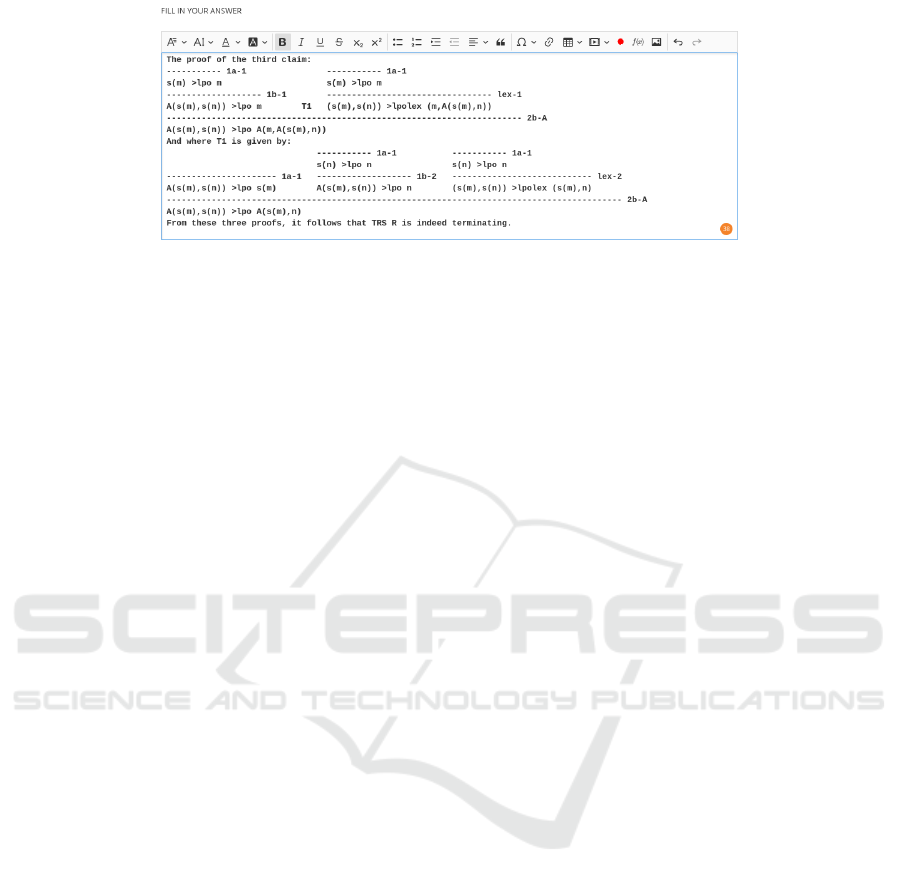
Figure 7: Tree style proof for the third claim created in Cirrus.
mented two question types that can be used for this
kind of questions, namely the ‘essay question’ and
the ‘file response question’. The last one basically
transforms the exam into a regular written exam, be-
cause students can write things on paper, take a pic-
ture of it, and upload it into Cirrus as an answer. This
works pretty well for ‘at home’ exams, but it usually
cannot be used for ‘on campus’ exams, because the
controlled circumstances disallow the usage of smart-
phones at all and there is no alternative available for
scanning student’s notes. Therefore, the focus in this
paper is about the usability of the ‘essay question’ for
submitting LPO proofs.
4.1 Natural Language Style Proofs in
Cirrus
When answering an ‘essay question’, students get a
‘rich text editor’ with the usual features like font se-
lection, markup like bold, italics, superscript and sub-
script, and lists, both with and without numbers. It
won’t be a surprise that this editor is suitable for typ-
ing proofs in natural language. Basically, the only
change is that it is probably wise to replace math-
ematical notation like >
lpo
and >
lex
lpo
by ‘>lpo’ and
‘>lpolex’ respectively, although even this can be ar-
ranged using the superscript and subscript options.
4.2 Tree Style Proofs in Cirrus
It may be a bit surprising, but within this editor
it is pretty well doable to create the trees in plain
ASCII. Again, replacing >
lpo
and >
lex
lpo
by ‘>lpo’ and
‘>lpolex’ respectively, makes it easier. In Figure 7
the tree for the proof of the third claim is included
as it is created inside of Cirrus. The main trick in
creating these trees easily within Cirrus is putting the
editor into a mono-spaced font. The fact that these
trees on paper are created bottom-up, is no problem,
because it is easy to insert new lines above the current
one. Aligning the different branches properly is also
easily established by inserting the proper amount of
spaces or dashes. So it is definitely doable to create
tree style proofs like this in Cirrus. A clear drawback
is that it takes quite some time.
4.3 Fitch Style Proofs in Cirrus
Whereas writing down Fitch proofs on paper has the
problems of guessing the amount of vertical space for
the subproofs and getting all the reference numbers
properly, in the rich text editor this is actually no prob-
lem at all. This is because of the automatically num-
bered lists. Simply start with the final goal as the first
item in a numbered list. In the proof of the third claim
this goal is proved by applying Rule 2b, which gives
three new proof obligations. Insert those above the
current goal and now the proof has four lines each
with their own unique label. In addition temporary
references I, II, and III can be added to the last line
because Rule 2b depends on those references. Those
temporary labels should also be added to the proof
obligations that they correspond to. As long as the
proof isn’t finished, the actual labels may still change
and therefore these temporary labels and references
are used. Once the proof is finished, all temporary
references can be replaced by the actual labels cor-
responding to the temporary labels. And of course,
all temporary labels can be removed. This process
is partially shown in Figure 8. Note that this exam-
ple provides also temporary labels for non-branching
steps. Of course, more experienced students will no-
tice that these are not really needed, because the final
reference will always be one line above in the situa-
tion where we do not optimize for having the same
proof obligations more than once.
Note that the Fitch style proof with hooks is not
easy to create in the rich text editor. If normal dashes
are used for showing the hooks, then the automatic
numbering is broken. However, it can be done by us-
ing the ‘underline’ option of the editor, but that takes
definitely more effort. We do not include the result in
CSEDU 2021 - 13th International Conference on Computer Supported Education
276

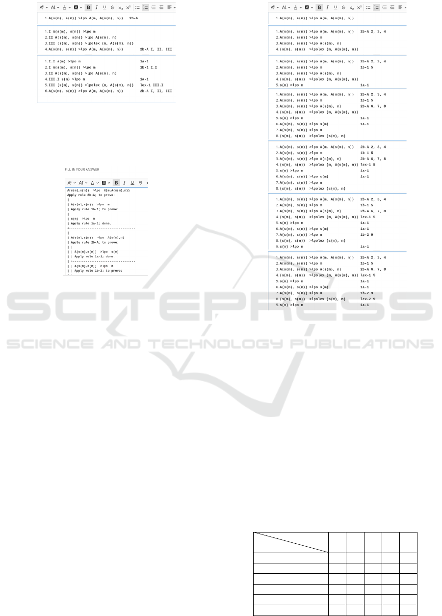
Figure 8: Step by step creation of a Fitch style proof for
the third claim in Cirrus. When the proof is complete all
temporary roman references can be replaced by the final line
numbers. The final result is an ASCII version of the proof
in Figure 3.
Figure 9: Partial Top-down Fitch style proof for the third
claim created in Cirrus.
this paper.
In contrast to this, the top-down Fitch style from
Figure 5 turns out to be pretty easy to format in the
rich text editor, because vertical and horizontal bars
can be typed directly in the editor. In addition, the
vertical space guessing problem is solved, because it
is easy to insert more space later on. The result is
presented in Figure 9.
However, the easiest method is probably the shuf-
fled Fitch proof. Figure 10 indicates how such a proof
can be created step by step. Note that we have intro-
duced a shortcut here to immediately add the proof
justification to a newly generated proof obligation
if this does not require any new proof obligations,
which is typically the case if we can prove a claim
by Rule 1a.
5 CONCLUSION
This paper is concluded by evaluating the proposed
proof styles with respect to the criteria that are impor-
tant in several educational contexts:
1. Do the proofs have an understandable structure
for the students?
Figure 10: Step by step creation in Cirrus of a shuffled Fitch
style proof for the third claim.
2. Can the proofs be constructed top-down in a sim-
ple way on paper?
3. Can the proofs be presented top-down in a simple
way on paper?
4. Can the proofs be constructed top-down in a sim-
ple way in a rich text editor?
5. Can the proofs be presented top-down in a simple
way in a rich text editor?
As can be seen in Table 1, there is no definitive ‘best
method’ that scores a plus on all criteria, but the top-
down Fitch style and the shuffled Fitch come close.
The only problem for the first one is the necessary
Table 1: Proof styles related to criteria.
Styles
Criteria
1 2 3 4 5
Natural language − ± + ± +
Tree + + − + −
Linear Fitch ± ± − + −
Hooked Fitch + ± − − −
Top-down Fitch + ± + + +
Shuffled Fitch ± + + + +
LPO Proofs in Two Educational Contexts
277

vertical space guessing when doing the proof on pa-
per. And the only problem for the latter one is the
lack of structure in the proof. However, the shuffled
Fitch style has an additional benefit that was not men-
tioned before: it is completely natural to write a sin-
gle proof in this style starting with all three claims for
the full proof, which is not the case for the top-down
Fitch style! The method will work in the same easy
way. So even though the shuffled Fitch style does not
clearly align with the nesting structure of the proof
method in general, it is very easy to present to stu-
dents as an algorithm. Therefore, this is probably the
best and certainly the most practical method for Com-
puting Science students to come up with a good, easy
to create, and easy to check LPO proof! If, on the
other hand, the focus is on the structure of the proof,
then the tree style proofs are probably the best pick,
especially for this group of students that has not seen
Fitch proofs before.
Note that this paper was specifically about LPO
proofs and about the digital exam environment Cir-
rus. However, the styles can be applied for basically
all mathematical proofs that rely on a series of ap-
plications of clear rules, and also in all other digital
assessment environments that have a reasonable rich
text editor.
6 FUTURE WORK
Because the idea for writing this paper only came up
after the exam and resit of the last time the course was
taught, there was no formal experiment conducted to
support the conclusions in Table 1, but instead gen-
eral impressions from the lectures, the input at the
exam (out of the eight students using LPO, one had
basically nothing, one tried a very informal natural
language proof, four had a formalized natural lan-
guage proof, one had a top-down Fitch style without
the lines, and one had both an informal natural lan-
guage proof and a top-down Fitch style without the
lines because he considered his own natural language
proof not clear enough), and private conversation with
students. In the next round of the course, also the
shuffled Fitch method will be introduced and students
will probably specifically be asked to use several LPO
proof visualizations in the homework and at the exam.
In addition, the question came up to give formal
semantics for the shuffled Fitch method and prove
that the method is sound and complete for this spe-
cific case where no normal ‘boxes’ are needed by
lack of real assumptions. It is also interesting to
check whether this shuffled Fitch method also works
for proofs that do use local assumptions. Using the
current informal semantics presented in Section 3.3,
this doesn’t seem likely because claims inside ‘boxes’
cannot typically be used outside these ‘boxes’.
ACKNOWLEDGEMENTS
The author thanks Cynthia Kop for comments on a
preliminary version and in particular for showing him
the so-called ‘shuffled Fitch style’ proof, which ac-
tually is the most innovative and promising method
discussed in this paper.
And the author thanks his wife for encouraging
him to finally write down some of his ideas forthcom-
ing from his teaching in this paper.
REFERENCES
Ackermann, W. (1928). Zum Hilbertschen Aufbau der
reellen Zahlen. Mathematische Annalen, 99(1):118–
133.
Baader, F. and Nipkow, T. (1998). Term rewriting and all
that. Cambridge University Press.
Cichon, E. and Marion, J.-Y. (2000). The Light Lexico-
graphic Path Ordering. CoRR, cs.PL/0010008.
Cirrus BV (2020). Cirrus Assessment. https://
cirrusassessment.com/.
Dershowitz, N. (1982). Orderings for term-rewriting sys-
tems. Theor. Comput. Sci., 17:279–301.
Kamin, S. and Levy, J.-J. (1980). Two Generalizations of
the Recursive Path Ordering. Technical report, Uni-
versity of Illinois, Urbana/IL.
Nordic Assessment Innovators (2020). Inspera Assessment.
https://www.inspera.com.
Paragin (2020). RemindoToets. https://www.paragin.nl/
remindotoets/.
Pelletier, F. J. (1999a). A Brief History of Natural Deduc-
tion. History and Philosophy of Logic, 20(1):1–31.
Pelletier, F. J. (1999b). A History of Natural Deduction and
Elementary Logic Textbooks.
P
´
eter, R. (1935). Konstruktion nichtrekursiver Funktionen.
Mathematische Annalen, 111(1):42–60.
Robinson, R. (1948). Recursion and Double Recur-
sion. Bulletin of the American Mathematical Society,
54:987–993.
Shelter, W. (1982). Maxima, a Computer Algebra System.
http://maxima.sourceforge.net/.
Sowiso BV (2020). SOWISO: A secure online testing and
learning environment for higher education math and
statistics. https://sowiso.nl/en.
Teelen (2020). TestVision. https://www.testvision.nl/en/.
Terese (2003). Term rewriting systems, volume 55 of Cam-
bridge tracts in theoretical computer science. Cam-
bridge University Press.
UNIwise (2020). WISEflow. https://www.uniwise.co.uk/
wiseflow.
Zantema, H. (2014). Berekeningsmodellen. Course notes.
CSEDU 2021 - 13th International Conference on Computer Supported Education
278