An Extreme Learning Machine based Approach for Software Effort

Estimation

Suyash Shukla and Sandeep Kumar

Department of Computer Science and Engineering, Indian Institute of Technology Roorkee, Roorkee, India

Keywords:

Software Effort Estimation, Machine Learning, Extreme Learning Machine.

Abstract:

Software Effort Estimation (SEE) is the task of accurately estimating the amount of effort required to develop

software. A signiﬁcant amount of research has already been done in the area of SEE utilizing Machine Learn-

ing (ML) approaches to handle the inadequacies of conventional and parametric estimation strategies and align

with present-day development and management strategies. However, mostly owing to uncertain outcomes and

obscure model development techniques, only a few or none of the approaches can be practically used for de-

ployment. This paper aims to improve the process of SEE with the help of ML. So, in this paper, we have

proposed an Extreme Learning Machine (ELM) based approach for SEE to tackle the issues mentioned above.

This has been accomplished by applying the International Software Benchmarking Standards Group (ISBSG)

dataset, data pre-processing, and cross-validation. The proposed approach results are compared to other ML

approaches (Multi-Layer Perceptron, Support Vector Machine, Decision Tree, and Random Forest). From the

results, it has been observed that the proposed ELM based approach for SEE is generating smaller error values

compared to other models. Further, we used the established approaches as a benchmark and compared the re-

sults of the proposed ELM-based approach with them. The results obtained through our analysis are inspiring

and express probable enhancement in effort estimation.

1 INTRODUCTION

Estimation of effort or cost required a develop soft-

ware is a tedious task in software project manage-

ment. In the past, the experts have battled a lot in

estimating the right amount of effort or cost, or du-

ration to complete the software. The estimation of

these parameters at the beginning phases of the soft-

ware development lifecycle is more troublesome be-

cause limits for each activity are required to set up,

and the functionalities for the end product are consid-

erable (Boehm, 1981). Most of the time, less infor-

mation about affecting variables and threats that may

happen, insistence from the customer or the execu-

tives, and traditional techniques of software estima-

tion may prompt incorrect results. Thus, they may se-

riously affect conveying project results inside a char-

acterized time allotment, ﬁnancial plan, and of satis-

factory quality. Despite the emergence of improved

software development methodologies, ongoing inves-

tigations of the Standish Group (2015) show that only

20% of projects are successful. The remaining 80%

of projects suffer from either the budget or time con-

straint, or the project won’t be able to meet the cus-

tomer satisfaction level, which results in the loss of

contracts and ﬁnancial loss.

As mentioned earlier, each activity of a project to-

ward the start of its lifecycle needs to deﬁne its cost

and calendar to decide a business plan and get the en-

dorsement from a customer. Purposefully, the expert

judgment technique that depends upon the knowledge

of estimators has been widely employed in the past

(Wysocki, 2014). But, these techniques usually lead

to errors. Therefore, various techniques based on Line

of Code (LOC) (Boehm, 1981) and Function Point

(FP) (Albrecht, 1979) have been introduced in the

past. The LOC and FP techniques have been modiﬁed

regularly to inherit the naive patterns in software de-

velopment methodologies and programming. Still, in

the quick-paced world of development, these proce-

dures are battling to stay up with the latest (Galorath

and Evans, 2006), particularly with advancing code

reuse and altered software deployment. Additionally,

they will generally be subjective, especially those de-

pendent on (Kemerer, 1993), and require considerable

effort for their usage and upkeep.

Consequently, a lot of research has been directed

to SEE utilizing machine learning methods (Sehra

Shukla, S. and Kumar, S.

An Extreme Learning Machine based Approach for Software Effort Estimation.

DOI: 10.5220/0010397700470057

In Proceedings of the 16th International Conference on Evaluation of Novel Approaches to Software Engineering (ENASE 2021), pages 47-57

ISBN: 978-989-758-508-1

et al., 2017) to handle the issues mentioned above.

These methods are considered exceptionally com-

pelling for handling vulnerability, and the got out-

comes present their incredible prediction capacities

for effort estimation at the underlying phases of the

lifecycle of the project (Berlin et al., 2009; Tronto

et al., 2008; Lopez-Martin et al., 2012). Also, through

their robotized estimation process dependent on past

data, they will, in general, lessen human inclinations

and mental or political impacts. Nevertheless, mostly

owing to uncertain outcomes and obscure model de-

velopment techniques, only a few or none of the ap-

proaches can be practically used for deployment. The

explanation for this may fall in limited research that

concentrated on ﬁnding the most exact ML strategy

and ﬁtting it for the best accuracy. Most of the re-

search has been done on the outdated and smaller

size datasets of ﬁnished projects, which tend to overﬁt

(Kocaguneli et al., 2012).

Furthermore, for data pre-processing, which is

considered important for creating successful mod-

els, different, often opposing techniques were applied

(Garc

ıa et al., 2016; Huang et al., 2015). On account

of the limitations sketched out above, there are un-

certain outcomes related to the performance of indi-

vidual methods, regardless of whether they were ap-

plied to a similar dataset. This could be a result of

various methodologies used by researchers or prac-

titioners for data pre-processing and developing ML

models for SEE.

This paper aims to improve the process of SEE

with the help of a powerful and handy approach. For

this purpose, we have proposed an Extreme Learn-

ing Machine (ELM) based approach for SEE to tackle

the issues mentioned above. This has been ac-

complished by applying the International Software

Benchmarking Standards Group (ISBSG) dataset,

data pre-processing, and cross-validation. The results

of the proposed approach are compared against four

other ML approaches, namely Multi-Layer Percep-

tron (MLP), Support Vector Machine (SVM), Deci-

sion Tree (DT), and Random Forest (RF). Further, we

used the established approaches as a benchmark and

compared the results of the proposed ELM-based ap-

proach with them.

Based on the above discussion, this research paper

aims the following research questions:

• RQ1: Which model is producing lesser error val-

ues for UCP estimation?

• RQ2: How much improvement/deterioration is

shown by the proposed ELM model for UCP esti-

mation compared to existing models?

To address these inquiries, an ELM based approach is

developed over the ISBSG dataset to estimate the ef-

fort required to develop software. Then, we compared

the proposed models performance with four other ML

models to obtain the best performing model. Further,

we compared the results of the proposed ELM-based

approach with the established benchmark approaches.

The rest of the paper is organized as per the fol-

lowing: In section 2, we discuss the overview of the

related work for SEE. In section 3, we discuss the pro-

posed approach for effort estimation. Results and sta-

tistical analysis are discussed in section 4 and section

5, respectively. Section 6 presents answers to the re-

search questions. Threats related to validity are dis-

cussed in section 7. Finally, section 8 presents the

conclusion.

2 RELATED WORK

The ML and data mining strategies have been exten-

sively utilized in the last two decades for software

estimation. The focus was to estimate the effort at

the initial phases since the estimation of these param-

eters at the beginning phases of the software devel-

opment lifecycle is more troublesome because of un-

certain and incomplete information. Any noteworthy

deviation of those requirements during the software

development lifecycle may seriously affect the func-

tionalities of the end product, its quality, and at last,

its successful completion.

In (Wen et al., 2012), they performed the most

thorough review of ML methods utilized for SEE.

They investigated 84 studies for this purpose. As indi-

cated by the outcomes, the researchers or practition-

ers concentrated more on ﬁtting single algorithms for

accurate results, especially; models based on Case-

Based Reasoning (CBR), decision trees, and Artiﬁ-

cial Neural Network (ANN). They found that the ML

models are more accurate compared to the traditional

models, with the value of Mean Magnitude Relative

Error (MMRE) lies in the range of 35-55%. They

also demonstrated that relying upon the dataset uti-

lized for developing ML models and the approaches

applied for data pre-processing, the ML models may

lead to contrast results due to noisy data and the prob-

ability of underﬁtting and overﬁtting.

The inconsistency in using various methodologies

for developing ML models for SEE is considerably

more noticeable while exploring individual studies.

For example, In (Tronto et al., 2008), the performance

of multiple regression models is compared against

the ANN model utilizing the COCOMO dataset, ex-

hibiting the superiority of the ANN model. They

used MMRE, and Percentage Relative Error Devia-

tion (PRED) measures to assess the performance of

ENASE 2021 - 16th International Conference on Evaluation of Novel Approaches to Software Engineering

developed models. In (L

opez-Mart

ın, 2015), vari-

ous types of neural networks are used to accurately

estimate the amount of effort required to develop

any software over the ISBSG dataset along with nor-

malization, cross-validation approaches, and different

performance evaluation measures. In (Berlin et al.,

2009), they adopted a progressively thorough strategy

concerning the scope and precision of Linear Regres-

sion (LR) and ANN models for effort as well as dura-

tion estimation. They utilized two datasets: a dataset

from the Israeli Company and ISBSG dataset. They

found that the performance of ANN was better than

LR and the accuracy improved by the log transforma-

tion of the target variables. Also, they demonstrated

that the effort estimation is more accurate compare to

duration estimation because the effort is more corre-

lated with the size variable.

In (Nassif et al., 2019), they adopted a regres-

sion fuzzy approach for the estimation of effort.

They utilized the ISBSG dataset of 468 projects

along with data preparation and cross-validation ap-

proaches. They utilized regression fuzzy models

for effort estimation. They found that the data het-

eroscedasticity affected the performance of ML mod-

els. They also found that the regression fuzzy logic

models are sensitive to outliers.

The data pre-processing step is very important

throughout the training process of ML models, par-

ticularly in managing outliers, the missing data which

largely affects the performance of ML models. In

(Huang et al., 2015), they suggested that aside from

the various deletion and imputation methods are avail-

able for data pre-processing, they are largely depen-

dent on the dataset. However, it is recommended to

discard the projects with missing values to decrease

the biases that affect ML models’ accuracy instead of

imputing them because imputation may reduce data

variability (Strike et al., 2001).

To evaluate the performance of effort estimation

models, most of the researchers use MMRE and

PRED (Wen et al., 2012). The assessment mea-

sures depend on different basic investigations, par-

ticularly MMRE, that is viewed as an asymmetric

measure (Myrtveit and Stensrud, 2012) and sensitive

to noise. Nonetheless, MMRE and PRED establish

an assessment standard, empower examination of re-

sults, and regularly with the help of Mean Absolute

Residual Error (MAR), Mean of Balanced Relative

Error (MBRE), Magnitude Relative Error to Estimate

(MMER), and Standardized Accuracy (SA) are still

generally utilized by researchers. Also, K-fold cross-

validation has been used widely to tackle the issue of

overﬁtting (Idri et al., 2016).

A few limitations are clear in the existing work.

Firstly, most of the investigations mentioned above

utilized small-sized datasets for model assessments.

It is a signiﬁcant downside since ML models’ accu-

racy may exceed expectations for the selected data

and decay large-sized data (Nassif et al., 2016). Sec-

ond, most of the existing studies have only used tra-

ditional ML models, especially ANN. The different

variants of the ANN model are needed to be explored

to get better results.

Moreover, most of the studies have used MMRE,

MMER, and PRED for assessing the performance of

the proposed models. Furthermore, only some of the

studies have used statistical tests to validate the per-

formance of their models. As indicated by (Myrtveit

and Stensrud, 2012), it is invalid to show one model’s

superiority over other models without doing proper

statistical analysis.

This paper aims to tackle the issues mentioned

above. For that reason, we developed an ELM based

model for SEE using the ISBSG dataset (2019 re-

lease) and compared its performance with four fre-

quently used existing ML models. Further, we com-

pared the results of the proposed ELM-based ap-

proach with the established benchmark approaches.

The statistical tests and assessment criteria proposed

by (Shepperd and MacDonell, 2012) are also used for

model validation.

3 PROPOSED APPROACH

A viable methodology dependent on best practices

and useful research discoveries for developing SEE

models utilizing ML algorithms is introduced in this

segment. Purposefully, the ISBSG dataset is used by

applying smart data pre-processing. Furthermore, the

acquired pre-processed data is applied to the mod-

elling of four ML models.

3.1 Data Preparation

Noisy data may seriously impact the performance of

ML models. A dataset in which the missing val-

ues and outliers are present in a signiﬁcant amount

is considered low-quality data, prompting inconsis-

tent results. So, data pre-processing is a basic assign-

ment during the development of ML models. This

study has used ISBSG release 2019 (ISBSG, 2019)

data to inspect ML models’ accuracy. As per (Jor-

gensen and Shepperd, 2007), using real-life projects

in SEE enhances the unwavering quality of the inves-

tigation. The 9178 projects developed using different

programming languages, and development paradigms

are present in this dataset.

An Extreme Learning Machine based Approach for Software Effort Estimation

3.1.1 Data Filtering

Provided the heterogeneous nature of the ISBSG

dataset and its huge size, a data pre-processing is

needed prior to performing any analysis. The rules

used for data ﬁltering are adapted from (Lokan and

Mendes, 2009) and shown in Table 1.

Table 1: Rules used for ﬁltering projects.

Criteria

Removed

Projects

Selected

Projects

Data quality

should be high

973 8205

Functional size

quality should

be high

1351 6854

No missing

value for the

development

team effort

720 6134

IFPUG 4+ is

used as a size

measure

1690 4444

Projects in this study are selected based on the fol-

lowing characteristics:

• High Data Quality: Each project in the ISBSG

dataset is assigned a data quality rating (A, B, C,

or D). For this study, we have only used projects

with data quality A or B.

• High UFP Quality: Each project in the ISBSG

dataset is assigned an unadjusted function point

(UFP) rating (A, B, C, or D). For this study, we

have only used projects with UFP quality A or B.

• Remove all the projects with missing develop-

ment team effort value.

• Remove all the projects in which the measure-

ment for size is other than IFPUG 4+. The IFPUG

projects are selected due to their popularity in the

industry.

3.1.2 Selected Features

The ISBSG dataset has three effort features: Sum-

mary Work Effort (SWE), Normalized Work Ef-

fort (NWE), and Normalized Work Effort Level 1

(NWEL1). The SWE is the most fundamental mea-

sure that represents the project’s complete effort in

terms of staff hours. Yet, SWE couldn’t cover all

the stages of the software development lifecycle. The

normalized effort is the total effort when missing

phases are added. However, there may be some ir-

regularities when using normalized effort because the

effort is reported based on various participants indi-

cated by resource level variable. The resource level

variable has four values: level 1 represents a devel-

opment team effort, level 2 represents an effort for

development team support, level 3 shows effort for

computer operations involvement, and level 4 shows

effort for end-users. Thus, to guarantee high consis-

tency, the utilization of NWEL1 as the target variable

has been suggested (Guevara et al., 2016), which is

chosen here.

Initially, the twenty most frequently used features

have been selected as independent features for ML

models (Guevara et al., 2016). The features with

missing values of more than 60% have been removed

from the initial set of 20 features. The removed fea-

tures are business area type, max team size, average

team size, input count, output count, enquiry count,

ﬁle count, and interface count. As mentioned above,

the NWEL1 is used as a dependent variable in this

study. The resource level value will be one for all

the projects because NWEL1 represents only the de-

velopment team’s effort. So, we have removed the

variable resource level from the initial set of features.

Hence, the dataset contains 4444 projects with 11 in-

dependent variables and one dependent variable.

This study has not used the two features, Applica-

tion Type (AT) and Organization Type (OT). Instead,

their derived versions, Application Group (AG) and

Industry Sector (IS) have been utilized to reduce their

complexity. Finally, the projects having missing val-

ues in any independent variable have been removed

from the dataset. The ﬁnal dataset has 927 projects

with 12 features. The independent variables used in

this study are shown in Table 2.

The statistical characteristics of the target variable

(NWEL1) are shown in Table 3. Also, before provid-

ing the dataset into the model, it is important to see

whether the input feature can be directly used in the

model or not. For instance, the DT is a categorical

feature. So, it can’t be used directly in the ML model.

For that reason, we performed one-hot encoding for

the encoding of the categorical variable. Since the

DT can take three values, the one-hot encoding pro-

cess will create three dummy variables. Similarly, we

perform one-hot encoding for other categorical vari-

ables, namely AG, 1DBS, DP, IS, LT, PPL, and UM.

3.2 Methodology

We have proposed an ELM based model for SEE. An

ELM model is an extension of a feed-forward neural

network (FFNN) model, which is in practice nowa-

days with good results. To the best of our knowl-

edge, an ELM model has not been used until now

ENASE 2021 - 16th International Conference on Evaluation of Novel Approaches to Software Engineering

Table 2: Independent variables used in this study.

Variable Description

Adjusted Function

Points (AFP)

Represents the size of the

software adjusted by the

Value Adjustment Factor

Application Group

(AG)

Groups the application type

into a set

1st Data Base

System (1DBS)

Shows the database for the

project

Development

Platform (DP)

PC, Mid-Range, Main

Frame, or Multi-

Platform

Development

Type (DT)

New, Enhanced, or Re-

development project

Functional Size

(FSZ)

Represents size in

adjusted function points

Industry Sector

(IS)

Represents organization

type responsible for

project submission

Language Type

(LT)

2G, 3G, 4G, or ApG

Project Elapsed

Time (PET)

Total time passed for

completing the project in

terms of calendar months.

Primary

Programming

Language (PPL)

The primary language

utilized for project

development.

Used Methodology

(UM)

Represents whether the

development methodology

is used or not.

Table 3: Statistical characteristics of effort variable in the

dataset.

Count 926

Mean 4893.91

Standard

Deviation

7803.52

Minimum 21

Maximum 88555

Median 2606

Skewness 5.04

Kurtosis 34.87

for the problem of SEE. Apart from that, we found

frequently used ML techniques for effort estimation

to compare the proposed ELM-based model’s per-

formance. The ML models used to compare the re-

sults of ELM based model are Multi-Layer Percep-

tron, Support Vector Machine, Random Forest, and

Decision Tree. We have implemented these ML mod-

els with 10-fold cross-validation and grid search ap-

proach to improve their performance. Further, the

accuracy estimates of these models are compared

against the benchmark model implemented over the

same dataset. The methodology used to develop these

ML models is shown in Figure 1.

The step by step methodology for SEE in this study is

explained below:

• Load Dataset: This step involves the loading of

raw data.

• Data Pre-processing: In this step, data cleaning

is done to make it suitable for the ML models.

In this study, several guidelines have been used

to handle missing data, as mentioned above. We

will have the ﬁnal dataset with 927 projects and

12 features at the end of this step.

• Train/Test Splitting: Divide each of the four

datasets into 80% training data and 20% testing

data.

• Apply ML Models: In this step, the dataset is

given as input to the ML models. The ML model

learns on train data and gives estimations for test-

ing data.

• Performance Evaluation: The error estimates of

different models on different datasets are evalu-

ated with different performance evaluation mea-

sures.

• Statistical Analysis: Then, the statistical analy-

sis is performed to compare the results of the pro-

posed models.

• Comparison with Benchmark Models: Finally,

the best performing proposed model’s error esti-

mates are compared against the benchmark mod-

els implemented over the same dataset.

4 EXPERIMENTAL ANALYSIS

4.1 Used ML Methods

ML algorithms are useful in extracting inherent data

patterns through automated learning over the input

(Ben-David and Shalev-Shwartz, 2014). The main

beneﬁt of ML algorithms over traditional methods is

that they can adapt well to the changing environment.

This property of ML algorithms is really useful for

SEE because, in the case of software, the technol-

ogy advancing by each passing day, na

ıve tools and

coding languages are accessible, and improved devel-

opment methodologies with a change in the skills of

the project development teams may affect the tradi-

tional SEE approaches. So, the problem of SEE is

complex, and ML algorithms are generally used to

model the complex relationship among the features

in the dataset.

An Extreme Learning Machine based Approach for Software Effort Estimation

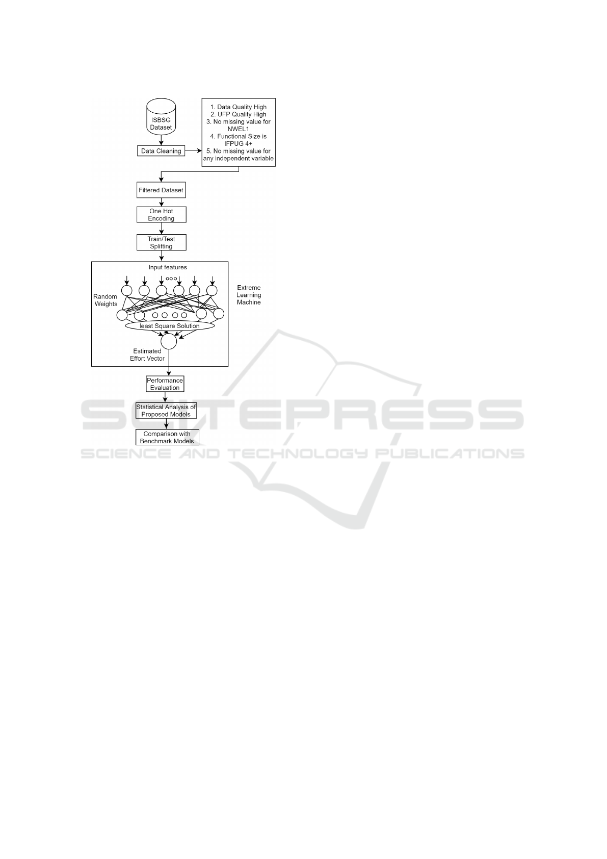
Figure 1: Proposed Methodology for SEE using ML mod-

els.

The ML algorithms are mainly categorized into

supervised and unsupervised algorithms. Countless

algorithms have been developed in the past under both

categories. This paper aims to estimate the effort re-

quired to develop software, and for that, we used ﬁve

ML algorithms ELM, SVR, MLP, DT, and RF.

SVM can model complex linear and nonlinear

problems and produces fewer error estimates, even

when the data contains outliers. This is because the

SVM utilizes kernels, and it won’t converge to local

minima (Han et al., 2006), whereas the MLP model

converges to local minima instead of global. The

MLP models performed well in noisy data because of

hidden layers and biases (Larose and Larose, 2015).

The MLP models are robust because of hidden layers

and biases. The DT model performs well for the noisy

datasets; they don’t require much data pre-processing

(Nie et al., 2011). So, they are useful for the ISBSG

dataset that contains many categorical variables with

lots of missing values and noise. The RF model is

almost similar to the DT model, except that the RF

model reduces overﬁtting and is more accurate to the

DT (Simone et al., 2016). The ISBSG dataset con-

tains noise and nonlinear variables; using these mod-

els can produce good results. The ANN model has

been studied a lot for SEE, but only traditional ANN

models have been used in most of the studies. The

different variants of the ANN model are needed to

be explored to get better results. The ELM model is

a type of neural network model which is very popu-

lar nowadays because of its super-fast nature. To the

best of our knowledge, the ELM model has not been

studied for SEE until now. Due to the reasons men-

tioned above, we decided to choose these models for

this study. The basics of these models are the follow-

ing:

4.1.1 ELM

ELM is an extension of the FFNN model with a sin-

gle hidden layer (Huang et al., 2011). The weights

for hidden neurons in the ELM model are assigned

randomly. The ELM models utilize the least square

regression method to predict the outcome. It is an

FFNN model, so data will go in a single direction,

and also, in ELM, the tuning of parameters is not re-

quired. The ELM model is famous for its simplic-

ity, super-fast computation, and unpredictable perfor-

mance. The ELM models are better than MLP and

other ANNs in terms of training time. The major limi-

tation of an ELM model is that it may lead to the prob-

lem of overﬁtting. Suppose a training sample (x

, t

)

is given, where x represents the input vector, t rep-

resents the output vector, i = 1...n, and n represents

the total training samples. The ELM model’s output

function with h hidden neurons can be mathematically

presented using equation 1.

(x) =

∑

i=1

∗a

(x) = Aβ (1)

Where A represents the hidden layer output matrix,

and β = [β

... β

]

represents the output matrix of

the ELM model.

A =







) a

) ... a

)

) a

) ... a

)

... ... ... ...

) a

) ... a

)







(2)

The output matrix β can be deﬁned using the follow-

ing equation:

β = A

∗Y (3)

Here, A

represents the Moore-Penrose generalized

inverse of matrix A and Y = [y

. . . y

]

is the target

matrix.

ENASE 2021 - 16th International Conference on Evaluation of Novel Approaches to Software Engineering

4.1.2 SVM

In the SVM technique, each data sample will be plot-

ted in the n-dimensional space as a data point, where n

depicts the number of input attributes (Drucker et al.,

1997). Then, the regression will be performed by

identifying the hyperplane. The hyperplane will help

us to predict the value of the target. In this method,

the main focus is on ﬁtting the error value inside some

threshold value, whereas in simple linear regression,

the aim was to reduce the amount of error. Based on

different kernel functions, the SVM method has three

variants; Linear SVM, Radial Basis Function (RBF)

SVM, and Polynomial SVM.

4.1.3 MLP

An MLP is a model that consists of at least three lay-

ers; 1 input layer, one hidden layer, and one output

layer (Murtagh, 1991). One can increase the num-

ber of hidden layers based on the complexity of the

task. The number of neurons in the input layer will be

equal to the number of input features. The number of

neurons in the output layer depends upon the type of

problem. The output of an MLP model for the regres-

sion problem will be a continuous value, and only one

neuron will be there in the output layer. If the value

predicted by the model differs from the actual value,

we will calculate the error and adjust the weights of

the model to reduce the amount of error.

4.1.4 DT

This model develops a tree-based model for classi-

ﬁcation as well as regression problems. The main

idea of this method is to predict the value of the tar-

get based on decision rules generated by the attributes

(Nie et al., 2011). This method divides the dataset

into smaller subsets and develops a related decision

tree at the time of division. The tree will be gener-

ated by recursive partitioning of each node. For tree

construction, knowledge of the domain is not required

and appropriate for the problem where enough infor-

mation is not available.

4.1.5 RF

The RF regression algorithm is an extension of the DT

algorithm. One of the DT algorithm’s main problems

is that they are very computationally expensive with

the risk of overﬁtting. Also, they are very much sen-

sitive to the training data samples. On changing the

training data, the predictions will be different. So, the

RF model combines various decision trees into one

to overcome the disadvantages of the decision tree

model (Simone et al., 2016).

4.2 Performance Evaluation Measures

• MAE: It is the average of actual and estimated val-

ues (Hardin et al., 2007).

MAE =

∑

i=1

−e

(4)

where, a

= actual values, e

= estimated values,

K= total number of samples.

• MBRE: It is the mean of the absolute error divided

by the minimum of actual and estimated values

(Hardin et al., 2007).

MBRE =

∑

i=1

min(a

, e

)

(5)

where,

−e

(6)

• MIBRE: It is the mean of the absolute error di-

vided by the maximum of actual and estimated

values (Hardin et al., 2007).

MIBRE =

∑

i=1

max(a

, e

)

(7)

• RMSE: It is calculated by taking the square root

of the mean of squared differences between actual

and estimated values (Satapathy and Rath, 2017).

MSE =

∑

i=1

−e

)

(8)

RMSE =

√

MSE (9)

• SA: It is calculated by taking the ratio of MAE

and MAE

(Azzeh and Nassif, 2016).

SA = 1 −

MAE

(10)

MAE

will be obtained by predicting the value

for the query utilizing many random sampling

runs over the remaining K-1 cases.

4.3 Results

In this study, the ELM model is designed to estimate

the effort required to develop software over the IS-

BSG dataset. Also, the error estimates of the pro-

posed ELM based model are compared against four

other models: SVR, MLP, DT, and RF. The ISBSG

dataset consists of 9178 projects with more than 100

features that contain noise and outliers. A dataset in

An Extreme Learning Machine based Approach for Software Effort Estimation

which the missing values and outliers are present in

a signiﬁcant amount is considered low-quality data,

prompting inconsistent results. So, the necessary

steps have been taken to remove the noise from the

data. After data processing, the dataset was left with

927 projects and twelve features. From the selected

927 projects, 80% of the projects were used for train-

ing, and the remaining 20% of the projects were used

for testing. The machine learning models have been

implemented with the help of a Scikit learn library in

python. 10-fold cross-validation and grid search ap-

proaches are used to ﬁnd the optimum parameters for

each model. After the model preparation and effort

prediction, the error estimates of proposed models are

evaluated based on different performance evaluation

measures. The results obtained after utilizing differ-

ent ML models on the ISBSG dataset are shown in

Table 4.

Table 4: Different error measures for effort estimation.

ELM SVM MLP DT RF

MAE 2310.7 2696.9 3580.2 3689.5 3599.5

RMSE 3350.8 4071.7 3311.4 3841.4 3432.4

MBRE 1.619 3.31 2.253 4.459 3.587

MIBRE 0.432 0.52 0.469 0.522 0.494

SA 60.10 53.43 38.18 36.29 37.84

From Table 4, we can say that the proposed ELM

model is performing well compared to the other mod-

els. The ELM is performing better than the other

models for all the accuracy measures. The MAE

value obtained by the proposed ELM based model is

2310.7. The DT model is the worst performing model

with an MAE value of 3689.5. The reason for the high

MAE values is that the dataset consists of heteroge-

neous projects and outliers. So, the outlier analysis

is also required for improving the performance of the

ML model.

5 STATISTICAL ANALYSIS

5.1 Comparison of Models

In the previous section, the error estimates of different

ML models on the ISBSG dataset are shown, and the

results show that the proposed ELM based approach

is efﬁcient for the SEE. Yet, the results of these ML

models are needed to be validated. So, we have per-

formed a statistical analysis on the estimated values

to investigate their statistical properties. We have se-

lected the Wilcoxon Rank test (Nassif et al., 2019) to

validate the proposed models’ performance based on

their estimated values. The Wilcoxon Rank test uses

to inspect whether two distributions are following the

same trend or not. The hypothesis for the test is the

following:

: No signiﬁcant difference among the two models

M1 and M2.

: The two models M1 and M2, are signiﬁcantly dif-

ferent.

The hypothesis mentioned above depends upon the

p-value. If the p-value exceeds 0.05, the model the

H0 will be accepted; otherwise, the hypothesis will

get rejected. The results of the Wilcoxon test for the

dataset are shown in Table 5.

Table 5: Wilcoxon Test Results for the Proposed ELM

Model.

P-value Nature

MLP 0.0678 Same

SVR 0.00 Different

RF 0.0037 Different

DT 0.0086 Different

Table 5 suggests that the ELM model is signif-

icantly different from the other models except for

MLP, whereas there is no signiﬁcant difference be-

tween MLP and ELM models.

5.2 Comparison with Benchmark

Models

The comparison of the best performing proposed

model has been made against the benchmark Fuzzy

and ANN models applied on the same datasets.In

(Nassif et al., 2019), they have used different fuzzy

logic models and multiple linear regression models.

They also compared the performance of the best per-

forming fuzzy logic model with the ANN model. Ta-

ble 6 shows the comparison of the proposed model

with the benchmark models based on similar accuracy

measures.

Table 6: Comparison of the proposed model with bench-

mark models based on different measures.

MAE MBRE MIBRE SA

Proposed ELM 2310.7 1.619 0.432 60.10

ANN Model

(Nassif et al., 2019)

5654.99 - - -

Fuzzy Model

(Nassif et al., 2019)

4925.23 1.761 0.609 55.1

MLR Model

(Nassif et al., 2019)

5536.3 3.192 0.497 49.6

From Table 6, it is clear that the proposed model

is better in comparison to the benchmark models.

The MAE estimates of the proposed ELM model are

half the MAE of the best performing ANN or Fuzzy

ENASE 2021 - 16th International Conference on Evaluation of Novel Approaches to Software Engineering

model. The MAE value for the ELM model is 2310.7,

whereas the MAE value for the fuzzy model 4925.23.

The reason for this difference may be the varying

sizes of datasets. They have used ISBSG release 11,

which was having nearly 6000 projects, whereas this

study based is conducted on the latest release of the

ISBSG dataset, which contains 9178 projects.

6 DISCUSSION

RQ1: Which machine learning model is generating

lesser error values for effort estimation?

To answer this research question, we have imple-

mented an ELM based model and applied it over the

ISBSG dataset and other frequently used ML models

for SEE studies. To evaluate the performance of these

models, we have used different performance evalua-

tion measures. Table 4 display the values of these per-

formance measures after applying above mentioned

ML models. By looking at the results, we can say that

the ELM model has outperformed the other ML mod-

els. The MAE obtained for the ELM model is 2310.7,

whereas the ELM has achieved 60.10% SA. To vali-

date the results of these models, we have conducted a

Wilcoxon Rank test to check whether the models have

a signiﬁcant difference or not. Based on the results,

we found that the ELM model is signiﬁcantly differ-

ent from every other model for the dataset except the

MLP model.

RQ2: How much improvement/deterioration is shown

by the proposed ELM model for effort estimation in

comparison to existing models?

To answer this research question, we have compared

the results of the proposed models with the bench-

mark ANN and fuzzy models develop over the same

dataset. Table 7 shows the comparison of the pro-

posed model with the benchmark models based on

MAE accuracy measures. From Table 7, we can say

that the proposed model is better than the benchmark

model. The proposed ELM model is better than the

fuzzy and ANN models in different error measures

values.

Table 7: Benchmark vs. proposed model comparison based

on different measures.

MAE MBRE MIBRE SA

Benchmark

Model

4925.23

(Fuzzy)

1.761

(Fuzzy)

0.609

(Fuzzy)

55.1

(Fuzzy)

Proposed

ELM Model

2310.7 1.619 0.432 60.10

Improvement/

Deterioration

53.08%

(imp)

8.06%

(imp)

29.06%

(imp)

Table 7 displays that the proposed model shows

an improvement of 53.08 for the ISBSG dataset in

terms of MAE. Here, imp stands for Improvement

7 THREATS TO VALIDITY

Internal Validity: As explained in the data pre-

processing step, the ISBSG data set consists of

projects in which the FP’s are used as the sizing meth-

ods. In this study also, only those projects have been

selected for which the sizing measure is IFPUG. Nev-

ertheless, the effect of other sizing measures on SEE

utilizing ML should be explored. But, setting up this

type of investigation is itself a challenging task be-

cause the data of good quality and reliability is not

easily available.

External Validity: The external validity questions

about the generalizability of results, whether the out-

comes of the research can be generalized or not. In

this study, we have used the ISBSG dataset with the

help of a smart data pre-processing approach. We

have also applied different ML models and evaluation

measures to assess the performance of applied ML

models. Finally, the results generated are validated

with the help of statistical analysis. So, we can say

the results of this study can be generalized up to an

extent. However, the results can improve more with

the help of more datasets.

8 CONCLUSIONS

Estimation of effort or cost required to develop soft-

ware is a tedious task in software project manage-

ment. Each activity of a project toward the start of

its lifecycle needs to deﬁne its cost and calendar to

decide a business plan and get the endorsement from

a customer. Purposefully, different traditional meth-

ods such as expert judgment and algorithmic meth-

ods have been developed in the past. But, in the

quick-paced world of development, these procedures

are battling to stay up with the latest. The ML algo-

rithms are useful in extracting inherent patterns from

the data through automated learning over the input.

The main beneﬁt of ML algorithms over traditional

methods is that they can adapt well to the changing

environment. This property of ML algorithms is re-

ally useful for SEE because, in the case of software,

the technology advancing by each passing day, na

ıve

tools and coding languages are accessible, and im-

proved development methodologies with a change in

the skills of the project development teams may af-

fect the traditional SEE approaches. A signiﬁcant

An Extreme Learning Machine based Approach for Software Effort Estimation

amount of research has already been done in SEE, uti-

lizing ML approaches to handle the inadequacies of

conventional and parametric estimation strategies and

align with present-day development and management

strategies. However, mostly owing to uncertain out-

comes and obscure model development techniques,

only a few or none of the approaches can be practi-

cally used for deployment.

This paper aims to improve the process of SEE

with the help of a powerful and handy approach. For

this purpose, we have proposed an ELM based ap-

proach for SEE to tackle the issues mentioned above.

This has been accomplished by applying the ISBSG

dataset. The ISBSG dataset contains 9178 projects

developed in different programming languages using

different development methodologies. So, this data

is heterogeneous data, which usually leads to incon-

sistent estimates. So, the necessary steps are needed

to remove the noise from the data. The projects in the

dataset have been ﬁltered based on data quality rating,

UFP rating, missing values in the dependent variable,

and missing values in independent variables. Here,

we have considered only those projects in which the

functional size is measured in IFPUG 4+. After per-

forming the data pre-processing, only 927 projects

were left with 12 features. Then, the acquired dataset

is given as input to the ML models.

The ML model learns on train data and gives esti-

mations for testing data. Then, the error estimates of

different models are evaluated with different perfor-

mance evaluation measures. By looking at the results,

we can say that the ELM model has outperformed the

other models, depending on the evaluation measures.

To validate the results of these models, we have con-

ducted a Wilcoxon Rank test to check whether the

models have a signiﬁcant difference or not. Based on

the results, we found that the ELM model is signiﬁ-

cantly different from every other model except MLP.

Finally, we compared the results of the proposed mod-

els with the benchmark ANN and fuzzy models de-

velop over the same dataset. Table 7 shows the com-

parison of the proposed model with the benchmark

models based on different accuracy measures. The

MAE values of the ELM model largely differ from

ANN and fuzzy models. The proposed model shows

an improvement of 53.08% compared to the bench-

mark fuzzy model.

In the future, it is recommended to use the more

advanced ML algorithms on some other datasets.

Also, the ISBSG dataset contains outliers that have

not been studied in this study. So, it’s recommended

to use different techniques to remove outliers from the

data to make it more useful for ML. The ISBSG data

without outliers may improve SEE analysis.

REFERENCES

Albrecht, A. (1979). Measuring application development

productivity. In In IBM Application Development

Symposium, pages 83–92.

Azzeh, M. and Nassif, A. (2016). A hybrid model for es-

timating software project effort from use case points.

Applied Soft Computing, 49:981–990.

Ben-David, S. and Shalev-Shwartz, S. (2014). Understand-

ing Machine Learning: From Theory to Algorithms,

Understanding Machine Learning: From Theory to

Algorithms. Cambridge University Press, New York.

Berlin, S., Raz, T., Glezer, C., and Zviran, M. (2009). Com-

parison of estimation methods of cost and duration in

it projects. Information and software technology jour-

nal, 51:738–748.

Boehm, B. W. (1981). Software Engineering Economics.

Prentice Hall, 10 edition.

Drucker, H., Burges, C., Kaufman, L., Smola, A., and Vap-

nik, V. (1997). Support vector regression machines.

In In Advances in neural information processing sys-

tems, pages 155–161.

Galorath, D. and Evans, M. (2006). Software Sizing, Es-

timation, and Risk Management. Auerbach Publica-

tions.

Garc

ıa, S., Luengo, J., and Herrera, F. (2016). Tuto-

rial on practical tips of the most inﬂuential data pre-

processing algorithms in data mining. Knowledge

based Systems, 98:1–29.

Guevara, F. G. L. D., Diego, M. F., Lokan, C., and Mendes,

E. (2016). The usage of isbsg data ﬁelds in software

effort estimation: a systematic mapping study. ournal

of Systems and Software, 113:188–215.

Han, J., Kamber, M., and Pei, J. (2006). Data Mining: Con-

cepts and Techniques. Morgan Kaufmann.

Hardin, J., Hardin, J., Hilbe, J., and Hilbe, J. (2007). Gen-

eralized linear models and extensions. Stata press.

Huang, G., Zhou, H., Ding, X., and Zhang, R. (2011). Ex-

treme learning machine for regression and multiclass

classiﬁcation. IEEE Transactions on Systems, Man,

and Cybernetics, Part B (Cybernetics), 42(2):513–

529.

Huang, J., Li, Y., and Xie, M. (2015). An empirical anal-

ysis of data preprocessing for machine learning-based

software cost estimation. Information and Software

Technology, 67:108–127.

Idri, A., Hosni, M., and Abran, A. (2016). Improved esti-

mation of software development effort using classical

and fuzzy analogy ensemble. Applied Soft Computing,

49:990–1019.

ISBSG (2019). International Software Benchmarking Stan-

dards Group.

Jorgensen, M. and Shepperd, M. (2007). A system-

atic review of software development cost estimation

studies. IEEE Transaction of Software Engineering,

33(1):33–53.

Kemerer, C. (1993). Reliability of function points measure-

ment: a ﬁeld experiment. In Commun. ACM 36, page

85–97.

ENASE 2021 - 16th International Conference on Evaluation of Novel Approaches to Software Engineering

Kocaguneli, E., Menzies, T., and Keung, J. (2012). On the

value of ensemble effort estimation. IEEE Transaction

of Software Engineering, 38:1402–1416.

Larose, D. and Larose, C. (2015). Data Mining and Predic-

tive Analytics. John Wiley & Sons, New Jersey.

Lokan, C. and Mendes, E. (2009). Investigating the use of

chronological split for software effort estimation. IET

Software, 3(5):422–434.

Lopez-Martin, C., Isaza, C., and Chavoya, A. (2012).

Software development effort prediction of industrial

projects applying a general regression neural network.

Empirical Software Engineering, 17:738–756.

opez-Mart

ın, C. (2015). Predictive accuracy comparison

between neural networks and statistical regression for

development effort of software projects. Applied Soft

Computing, 27:434–449.

Murtagh, F. (1991). Multilayer perceptrons for classiﬁ-

cation and regression. Neurocomputing, 2(5-6):183–

197.

Myrtveit, I. and Stensrud, E. (2012). Validity and reliabil-

ity of evaluation procedures in comparative studies of

effort prediction models. Empirical Software Engi-

neering, 17:23–33.

Nassif, A., Azzeh, M., Capretz, L., and Ho, D. (2016). Neu-

ral network models for software development effort

estimation: a comparative study. Neural Computing

and Applications, 27(8):2369–2381.

Nassif, A., Azzeh, M., Idri, A., and Abran, A. (2019). Soft-

ware development effort estimation using regression

fuzzy models. Computational intelligence and neuro-

science.

Nie, G., Rowe, W., Zhang, L., Tian, Y., and Shi, Y. (2011).

Credit card churn forecasting by logistic regression

and decision tree. Expert Systems with Applications,

38(12):15273–15285.

Satapathy, S. and Rath, S. (2017). Empirical assessment of

ml models for effort estimation of web-based appli-

cations. In In Proceedings of the 10th Innovations in

Software Engineering Conference, page 74–84.

Sehra, S., Brar, Y., Kaur, N., and Sehra, S. (2017). Research

patterns and trends in software effort estimation. In-

formation and software technology journal.

Shepperd, M. and MacDonell, S. (2012). Evaluating pre-

diction systems in software project estimation. Infor-

mation and Software Technology, 54(8):820–827.

Simone, P., Alessandrlo, M., Demeyer, S., Marchesi, M.,

and Tonelli, R. (2016). Estimating story points from

issue reports. In In Proceedings of the 12th Interna-

tional Conference on Predictive Models and Data An-

alytics in Software Engineering, pages 1–10.

Strike, K., Emam, K., and Madhavji, N. (2001). Software

cost estimation with incomplete data. IEEE Transac-

tion of Software Engineering, 27:890–908.

Tronto, I. D. B., Silva, J. D., and Anna, S. (2008). An inves-

tigation of artiﬁcial neural networks based prediction

systems in software project management. Journal of

Systems and Software, 81:356–367.

Wen, J., Li, S., Lin, Z., Hu, Y., and Huang, C. (2012). Sys-

tematic literature review of machine learning based

software development effort estimation models. In-

formation and Software Technology, 54:41–59.

Wysocki, R. (2014). Effective Project Management: Tradi-

tional, Agile, Extreme, Industry Week. John Wiley &

Sons.

An Extreme Learning Machine based Approach for Software Effort Estimation