On the Improvement of Feature Selection Techniques: The Fitness Filter

Artur J. Ferreira

1,3 a

and M

ario A. T. Figueiredo

2,3 b

ISEL, Instituto Superior de Engenharia de Lisboa, Instituto Polit

ecnico de Lisboa, Portugal

IST, Instituto Superior T

ecnico, Universidade de Lisboa, Portugal

Instituto de Telecomunicac¸

oes, Lisboa, Portugal

Keywords:

Machine Learning, Feature Selection, Dimensionality Reduction, Relevance-Redundancy, Classiﬁcation.

Abstract:

The need for feature selection (FS) techniques is central in many machine learning and pattern recognition

problems. FS is a vast research ﬁeld and therefore we now have many FS techniques proposed in the liter-

ature, applied in the context of quite different problems. Some of these FS techniques follow the relevance-

redundancy (RR) framework to select the best subset of features. In this paper, we propose a supervised

ﬁlter FS technique, named as ﬁtness ﬁlter, that follows the RR framework and uses data discretization. This

technique can be used directly on low or medium dimensional data or it can be applied as a post-processing

technique to other FS techniques. Speciﬁcally, when used as a post-processing technique, it further reduces

the dimensionality of the feature space found by common FS techniques and often improves the classiﬁcation

accuracy.

1 INTRODUCTION

The goal of feature selection (FS) can be stated as that

of ﬁnding the best subset of features for a given prob-

lem (Duda et al., 2001; Guyon et al., 2006; Guyon and

Elisseeff, 2003). The use of FS techniques mitigates

the effects of the “curse of dimensionality” (Bishop,

1995; Bishop, 2007) phenomenon and it improves the

accuracy of machine learning tasks.

In the past years, with the advent of big data and

as a consequence high-dimensional data being often

present for many problems, the use of FS techniques

is an important and active topic of research. In the

presence of high-dimensional data, the irrelevance of

many features and the redundancy among features is

often found. For many years, researchers in the ma-

chine learning and pattern recognition ﬁelds have car-

ried investigation efforts to develop adequate FS tech-

niques for many different problems. As a result from

these research efforts, we now have many FS tech-

niques available and suited for quite different prob-

lems, within research ﬁelds and applications such as

data mining, computer vision, and biomedical data.

Some of the existing FS techniques aim at ﬁnding

the relevant features, while discarding the irrelevant

https://orcid.org/0000-0002-6508-0932

https://orcid.org/0000-0002-0970-7745

and redundant ones. However, in some cases, the use

of one single FS technique on the input data yields

sub-optimal solutions, regarding the size of the re-

sulting subset and the remaining redundancy among

features. In many of these situations, this results

from non-optimal parametrization of the FS algorithm

used. It is also known from the literature that the use

of discretization of the data typically improves on the

performance of machine learning and data mining al-

gorithms. The use of feature discretization (FD) tech-

niques usually yields more compact feature subsets

with better performance, as compared to the use of

the original features (Garcia et al., 2013).

In this paper, we propose a supervised ﬁlter fea-

ture selection technique named as ﬁtness ﬁlter (FF).

This technique can be used directly on low or medium

dimensional data or it can be applied as a post pro-

cessing technique after the use of another FS algo-

rithm. In both scenarios, FF attains adequate results

at reducing the dimensionality of the data.

The remainder of this paper is organized as fol-

lows. Section 2 overviews FS ﬁlter approaches with

the RR framework. The proposed FF technique is pre-

sented in Section 3 and evaluated in Section 4. Fi-

nally, Section 5 ends the paper with some concluding

remarks and directions for future work.

Ferreira, A. and Figueiredo, M.

On the Improvement of Feature Selection Techniques: The Fitness Filter.

DOI: 10.5220/0010396303650372

In Proceedings of the 10th International Conference on Pattern Recognition Applications and Methods (ICPRAM 2021), pages 365-372

ISBN: 978-989-758-486-2

365

2 FEATURE SELECTION

The need for FS often arises in many machine learn-

ing problems. The use of a FS technique usually im-

proves the accuracy of a classiﬁer learnt from data,

since it helps to mitigate the effects of the well-

known “curse of dimensionality”. By removing some

features from the original data, we have a speed-

up of the training time and an improvement of the

generalization ability of a classiﬁer. Thus, the re-

search community has developed many methods to

perform FS. In Subsection 2.1, we review some as-

pects and taxonomy regarding FS techniques. The

contents of Subsection 2.2 refer to the relevance-

redundancy framework, which is the foundation of

our proposal in this paper. Subsection 2.3 brieﬂy de-

scribes some successful supervised FS ﬁlters that re-

sort to the relevance-redundancy framework. Finally,

Subsection 2.4 brieﬂy reviews the beneﬁts of using

discretized data on FS methods.

2.1 Notation and Concepts

We start by introducing some notation. Let X =

,... ,x

} be a dataset, with n patterns/examples.

Each pattern x

is a d-dimensional vector, thus d de-

notes the number of features, that is, the dimension-

ality of the data. The dataset X can be seen as n × d

matrix, in which the rows hold the patterns and the

columns are the features, designated as X

. Let c de-

note the number of distinct class labels represented

by c

and y = {c

,. .. ,c

} is the class label vector. FS

techniques can be placed into one of four categories:

wrapper, embedded, ﬁlter, and hybrid. For recent sur-

veys on FS techniques, please see (Chandrashekar and

Sahin, 2014) and (Miao and Niu, 2016).

2.2 Relevance-Redundancy

The relevance-redundancy (RR) framework (Peng

et al., 2005; Yu and Liu, 2004; Ooi et al., 2005; Zhang

et al., 2006) is followed by some FS methods. Let S

be some subset of selected features and p(c|S) be the

conditional probability of the class given S. The con-

cepts of relevance and redundancy can be formalized

as follows (John et al., 1994):

• a feature X

/∈ S is said to be relevant iff p(c|S) 6=

p(c|S,X

); otherwise, feature X

is considered as

irrelevant;

• a feature X

/∈ S is said to be redundant iff

p(c|X

,S) = p(c|S), and p(c|X

) 6= p(c|S

), with

being a subset of S.

Thus, a feature X

is considered relevant, if its con-

catenation to the current feature set S, changes the

conditional probability of the class given the result-

ing feature set. A feature is redundant, in the pres-

ence of others, when there exists a smaller subset of

features holding the same the conditional probability

of the class given the feature set. However, this fea-

ture can be added to a smaller subset, without degrad-

ing this conditional probability. A feature can become

redundant due to the existence of other relevant fea-

tures, which provide similar prediction power. In this

case, it is of no worth to add a redundant feature to

the existing subset of features.

The RR framework for FS aims to remove the

redundant features, while keeping the most relevant

ones, thus expecting to improve the prediction accu-

racy. In (Yu and Liu, 2003; Yu and Liu, 2004), it is

shown that feature relevance alone is insufﬁcient for

a good performance of FS methods, when the dimen-

sionality of the data increases. Therefore, redundancy

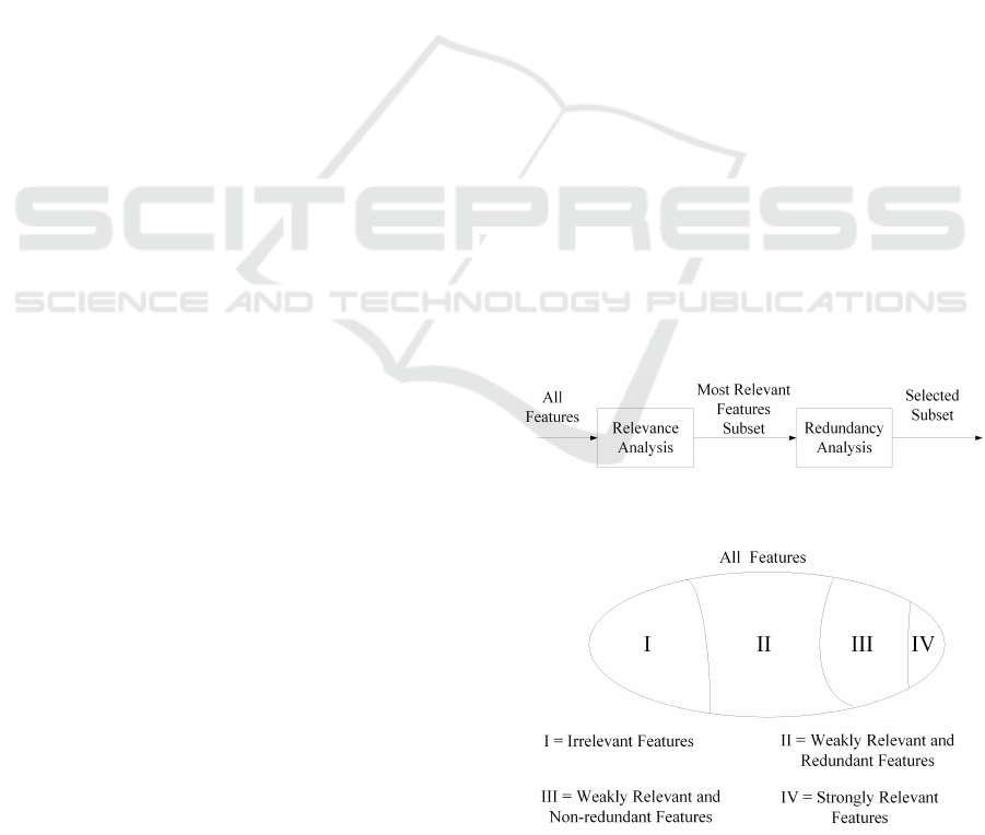
analysis is also necessary. Figure 1 depicts the RR

framework approach with two key steps:

(1) compute the relevance of each feature (or a subset

of features) and sort the resulting values into a list

by decreasing order, keeping the most relevant;

(2) remove the redundant features from the list.

Thus, we check for redundancy among the most rele-

vant features. In high-dimensional data, features can

be categorized into four subsets (Yu and Liu, 2004),

as depicted in Figure 2. A FS technique should ﬁnd

the subset composed by both the weakly relevant and

the non-redundant features (part III) and the strongly

relevant features (part IV).

Figure 1: The relevance-redundancy framework key steps

for feature selection, as proposed by (Yu and Liu, 2004).

Figure 2: Feature categorization, as proposed by (Yu and

Liu, 2004). The optimal subset of features is given by part

III + part IV. Notice the size proportion between the subsets.

ICPRAM 2021 - 10th International Conference on Pattern Recognition Applications and Methods

366

2.3 Supervised Filter Methods

In this Subsection, we brieﬂy describe three success-

ful supervised ﬁlter FS techniques that follow the RR

framework, as depicted in Figure 1, and have been

proven effective for many machine learning problems.

The maximal relevance minimum redundancy

(MRMR) method (Peng et al., 2005) computes both

the redundancy between features and the relevance of

each feature. The relevance is measured by the mutual

information (MI) between each feature and the class

labels. The redundancy between pairs of features is

also computed by MI. For two discrete random vari-

ables, U and V , MI is deﬁned as

MI(U ;V ) =

∑

i=1

∑

j=1

U,V

(i, j) log



U,V

(i, j)

(i)p

( j)



(1)

in which p

U,V

(i, j) is the joint probability of U and V .

MI is non-negative, being zero only when U and V are

statistically independent (Cover and Thomas, 2006).

The fast correlation-based ﬁlter (FCBF) was pro-

posed in (Yu and Liu, 2003; Yu and Liu, 2004). The

algorithm computes the feature-class and the feature-

feature correlations. It starts by selecting a set of fea-

tures that is highly correlated to the class with a cor-

relation value above some threshold set by the user.

The features with higher correlation with the class are

called predominant, in the ﬁrst step. This correlation

is assessed by the symmetrical uncertainty (SU) (Yu

and Liu, 2003) measure, deﬁned as

SU(U,V ) =

2MI(U ;V )

H(U) + H(V )

, (2)

where H(.) denotes the Shannon entropy of the ran-

dom variable (Cover and Thomas, 2006). The SU is

zero for independent random variables and one for de-

terministically dependent random variables.

In the second step, a redundancy detection proce-

dure ﬁnds redundant features among the predominant

ones. The set of redundant features is further split in

order to remove the redundant ones and keep those

that are the most relevant to the class. In order to re-

move the redundant features, three heuristic criteria

are applied.

The relevance-redundancy feature selection

(RRFS) method (Ferreira and Figueiredo, 2012)

follows the RR framework. RRFS, ﬁrst ﬁnds the

most relevant subset of features and then searches for

redundancy among some pairs of the most relevant

features. In the end, it keeps only features with high

relevance and low redundancy among themselves

(below some threshold, named as maximum sim-

ilarity, M

). RRFS uses a generic (unsupervised

or supervised) relevance measure and the abso-

lute cosine between feature vectors to assess the

redundancy.

2.4 The Beneﬁts of Discrete Data

Many datasets have features with continuous (real)

values. The use of feature discretization (FD) tech-

niques aims to yield representations of each feature

that contain enough information for the subsequent

machine learning task, discarding minor ﬂuctuations

that may be irrelevant (Garcia et al., 2013; Garcia

et al., 2016). Thus, the use of FD techniques aims at

ﬁnding compact and more adequate representations of

the data for learning purposes. The use of FD usually

leads to a set of features yielding both better accu-

racy and lower training time, as compared to the use

of the original features. It has been found that the

use of FD techniques, with or without a coupled FS

technique, may improve the results of many learning

methods (Witten et al., 2016).

Moreover, some machine learning and classiﬁ-

cation algorithms can only deal with discrete fea-

tures, thus at a certain point a discretization proce-

dure is necessary in these cases, as a pre-processing

stage (Hemada and Lakshmi, 2013).

3 FITNESS FILTER

In this section, we present in detail the proposed ﬁt-

ness ﬁlter (FF) method. Subsection 3.1 describes the

key ideas behind the proposal of the method. Sub-

section 3.2 presents the FF method in an algorithmic

style and ﬁnally Subsection 3.3 shows some analysis

on the ﬁtness and redundancy values for two datasets.

3.1 The Key Ideas

The FF method is tailored to be applied in two differ-

ent scenarios:

(i) direct use on the input data - acting as a supervised

FS ﬁlter, suited for low and medium dimensional

datasets, with, say, d < 100;

(ii) as a post-processing technique that further re-

duces the size of the subset of features found by

(any) common FS method.

The method relies on the RR framework as depicted

in Figure 1, in the sense that it computes the ﬁtness

of each feature as the sum of its relevance to the class

label vector, subtracted by the average redundancy of

the feature, in the presence of all the other features.

On the Improvement of Feature Selection Techniques: The Fitness Filter

367

The goodness of a feature X

is directly proportional

to the value of its ﬁtness, given by

f (X

) = rel(X

,y)

| {z }

relevance

−

d − 1

∑

j=1 j6=i

red(X

)

| {z }

redundancy

, (3)

where:

(i) rel(X

,y) denotes the relevance of feature X

, re-

garding the class label vector y; rel(.) is a generic

relevance function;

(ii) red(X

) denotes the redundancy among the

pair of features X

and X

; red(.) is a generic re-

dundancy (similarity) function.

These functions are generic and thus we can chose

different ways to compute the relevance and the re-

dundancy. However, care must be taken on the dy-

namic range of the values produced by these mea-

sures. The rel(.) and red(.) functions should return

non-negative values on the same range, e.g. 0 to r,

for instance with r = 1. When using functions that

do not produce values in the same range, then it is

necessary to apply some normalization in order to as-

sure that both functions meet this requirement. For

instance, the MI and the SU measures presented in

equations (1) and (2), respectively, are adequate for

this purpose. Moreover, other quantities from infor-

mation theory can also be applied.

As described in Subsection 2.4, there are many

beneﬁts of using discrete data for learning tasks.

Thus, the proposed FF method uses a supervised FD

algorithm,

= disc(X

,y), that discretizes individu-

ally each feature X

, given the class label vector y.

This is the ﬁrst step of the algorithm and it aims to

attain an adequate representation of the data, before

the ﬁtness is computed for each feature. There are

many adequate supervised FD algorithms in the liter-

ature (Garcia et al., 2013).

3.2 The Algorithm

The generic proposed technique is presented as Al-

gorithm 1. After computing the ﬁtness of each fea-

ture, the algorithm keeps those with ﬁtness above the

fit parameter. By assuring that the rel(.) and red(.)

functions output values in the same range, the mid-

point 0 may be a meaningful crossing point to assess

the goodness of each feature. A zero-ﬁtness feature

means that the amount of relevance of that feature

equals the average redundancy of that feature with

all the features. Regarding the choice of the disc(.),

rel(.), and red(.) functions, we recommend the fol-

lowing:

Algorithm 1: Fitness Filter (supervised).

Input: X, n × d matrix, n patterns of a d-dimensional

training set.

y, 1 × n class label vector.

disc(.), a discretizer function.

rel(.), a relevance function.

red(.), a redundancy function.

f it, the minimum ﬁtness threshold.

Output: idx: m−dimensional vector with the indexes of

the selected features.

1: Discretize each feature

= disc(X

,y), (columns of

X), for i ∈ {1, ..., d}, obtaining a discretized version

of the training data.

2: Compute the ﬁtness of each feature f (

) (columns of

X), for i ∈ {1, ..., d}, using equation (3), with appro-

priate rel(.) and red(.) functions.

3: idx ← Keep the indexes of the features, for which

f (

) ≥ f it.

• disc(.) - a supervised discretizer using measures

from statistical or information theory to compute

the discretization bins; for instance, the well-

known method by (Fayyad and Irani, 1993);

• rel(.) and red(.) - a statistical measure of resem-

blance, such as correlation coefﬁcients or indexes;

a measure from information theory such as MI or

SU, as deﬁned in equations (1) and (2), respec-

tively.

3.3 Fitness and Redundancy Analysis

In order to get some insight into how the ﬁtness and

redundancy values change for different datasets, Fig-

ure 3 shows the ﬁtness values, computed as in (3) and

the red values using MI, for the Dermatology and

Lung datasets (described in Table 1). On the left-

hand-side, we have the ﬁtness values for the d = 34

features, while on right-hand-side, we have the re-

dundancy values for all pairs of features, displayed

as a d × d image (the main diagonal corresponds to

the similarity of a feature with itself). We consider

MI for both rel and red functions. We have distinc-

tive ﬁtness values, with all of the features exhibiting

positive values. On the redundancy analysis, we can

identify small groups of features as being more sim-

ilar between themselves and thus may be redundant

for a given learning task. For the Lung dataset, we ob-

serve a much more distinctive variation on the ﬁtness

values, since in this case only m = 27 features have

a positive ﬁtness value. The redundancy pattern (the

right-hand-side image) is also quite different from the

corresponding image on the Dermatology dataset.

ICPRAM 2021 - 10th International Conference on Pattern Recognition Applications and Methods

368

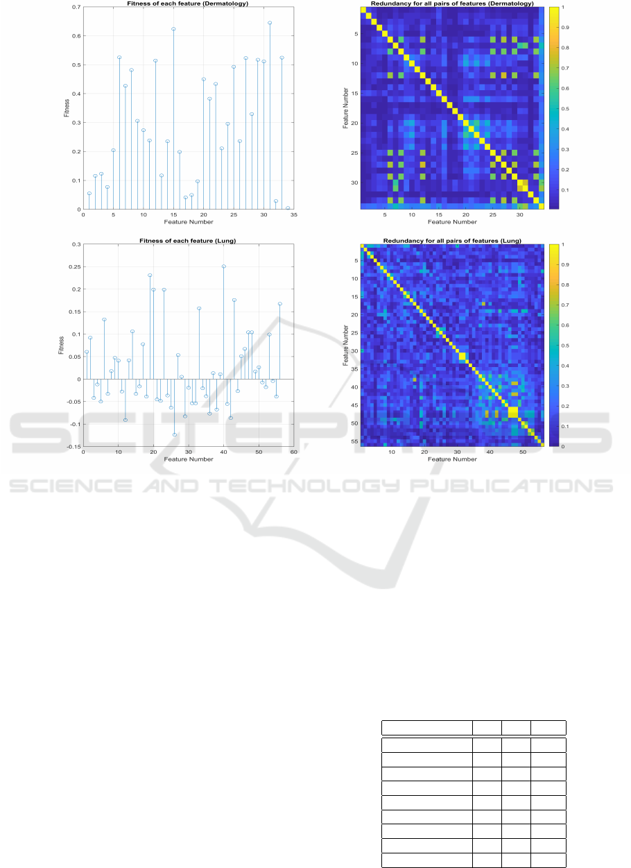
Figure 3: Fitness and redundancy of all the features: top - Dermatology dataset (d = 34); bottom - Lung dataset (d = 56).

4 EXPERIMENTAL EVALUATION

In this section, we report the experimental evaluation

of the proposed method. Subsection 4.1 describes

the public domain datasets considered on the experi-

ments. The learning task and its assessment measures

are described in Subsection 4.2. On Subsection 4.3

and Subsection 4.4, we report some experimental re-

sults on standard datasets, on the two scenarios de-

scribed in Section 3.1.

4.1 Public Domain Datasets

Table 1 brieﬂy describes the public domain bench-

mark datasets from the University of California

at Irvine (UCI) (Dua and Graff, 2019) and the

knowledge extraction based on evolutionary learning

(KEEL) repositories (Alcal

a-Fdez et al., 2011), which

were considered in our experiments. We chose several

well-known datasets with different kinds of data.

4.2 Learning Task and Assessment

As the learning task for the assessment of the pro-

posed FF method, we have considered the super-

vised classiﬁcation scenario. We use the linear sup-

port vector machine (SVM) classiﬁer, implemented

in the Waikato environment for knowledge analysis

(WEKA) tool (Frank et al., 2016). The classiﬁca-

Table 1: UCI and KEEL datasets used in our experiments;

d, c, and n denote the number of features, classes, and pat-

terns, respectively.

Dataset Name d c n

Heart 13 2 270

Wine 13 3 178

Hepatitis 19 2 155

WBCD 30 2 569

Dermatology 34 6 358

Ionosphere 34 2 351

Lung 56 3 32

Sonar 60 2 208

Libras 90 15 360

On the Improvement of Feature Selection Techniques: The Fitness Filter

369

tion accuracy of the classiﬁers were evaluated using

a leave-one-out cross-validation (LOOCV) method-

ology. We have also considered the implementation

of the FS methods available at the Arizona State Uni-

versity (ASU) repository for FS (Zhao et al., 2010),

with their parameters set with the corresponding de-

fault values.

In our experiments, we have made the following

choice of functions for the FF method:

• disc(.) - the supervised discretization method

by (Fayyad and Irani, 1993), named as informa-

tion entropy maximization (IEM), with its default

parameter values;

• rel(.) and red(.) - the SU as deﬁned in equa-

tion (2).

4.3 Direct Use on the Input Data

We start by analyzing the sensitivity of the FF method

with the changes on the fit parameter value in Fig-

ure 4. We display the test set error for the SVM clas-

siﬁer, using the LOOCV methodology, for different

values of the fit parameter. We compare the test er-

ror with the original baseline and the discretized (with

IEM) baseline dataset, for the SVM classiﬁer.

For the Hepatitis dataset, we have that ﬁt=-0.08 is

the optimal choice for the minimum test set error rate

and for fit values below 0.04, we attain lower test

error rate, as compared with the full set of features.

On the Dermatology dataset the optimal ﬁt values are

0.04 and 0.05, to attain the lowest test set error rate.

On the Ionosphere dataset, it is not possible to achieve

lower test error rate, as compared with the full set of

features. However, using the chosen selected subsets

of features by FF for fit up to -0.01, the test error is

never worse than using the full set of features. For the

Sonar dataset, the optimal value for the fit parame-

ter is below -0.1. For all datasets, an excessive large

value of the fit parameter will lead to a reduced sub-

set size and as a consequence to a low test set error

rate.

We now consider the use of the FF method, as

compared to the MRMR, FCBF, and RRFS methods,

described in Section 2.3, to perform FS on low and

medium dimensional datasets. Thus, we perform a

comparison of these methods for the supervised FS

ﬁlter task. For each dataset, the FCBF method is used

ﬁrst, with its default parameters, and it returns the

subset of features, with m features. Then, MRMR and

RRFS methods are applied using m as the size of the

subset of features to be selected, for a fair comparison.

Table 2 reports the experimental results for the SVM

classiﬁer. The column entitled ‘Original’ means that

we consider all the features (the original dimensional-

ity of data), and ‘Original Q.’ means their discretized

(quantized) version with the IEM algorithm.

4.4 Post-processing

On the second set of experiments, we apply the FF

method after the use of the FCBF and RRFS methods

on the input data. We aim to check if the use of the

FF method further improves on the results of the ﬁrst

FS method. Table 3 shows the results obtained by the

SVM classiﬁer on the FCBF and RRFS methods with

and without improvement with FF. From these results,

we conclude that:

• The discretization step improves the test error

rate, for most datasets.

• The FF method after the FS ﬁlter never gets a

worst result than the ﬁrst method. In some cases,

it also improves the results, like in the Heart

dataset (FCBF-FF provides the same test error

rate as FCBF, but using less features).

5 CONCLUSIONS

The development of feature selection techniques to

ﬁnd adequate subsets of data adequate for machine

learning problems is an active research ﬁeld, since

many problems in different domains require their use.

The relevance-redundancy framework is suited to ad-

dress the taxonomy of the feature subspaces and to

be used as a foundation to develop successful feature

selection methods and approaches. Along the years,

some feature selection methods based on this frame-

work have been proposed, aiming to keep the relevant

features, while discarding the irrelevant and redun-

dant ones. When using these methods, after the fea-

ture selection stage, there are still some redundancies

on the remaining subset of features, in some cases.

In this paper, we have proposed a new supervised

ﬁlter method based on the relevance-redundancy

framework, that can further reduce the dimensionality

of the data, after the use of a common feature selec-

tion method. The proposed method is also adequate

to be directly applied on the data, for low and medium

dimensional datasets, since the redundancy check part

of the algorithm has nearly quadratic complexity with

the dimensionality of the data.

The experimental results using public domain

datasets and standard methodologies have shown that

the proposed approach attains adequate results, being

competitive with state-of-the art methods. The pro-

posed approach is also able to successfully reduce the

data dimensionality.

ICPRAM 2021 - 10th International Conference on Pattern Recognition Applications and Methods

370

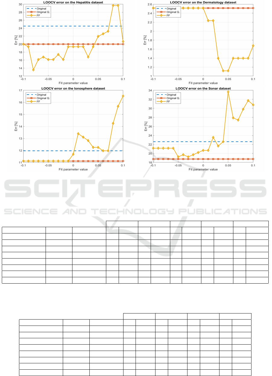
Figure 4: Test set error of the SVM classiﬁer, using the LOOCV methodology, with the original, original IEM discretized

data, and FF on the Hepatitis, Dermatology, Ionosphere, and Sonar datasets.

Table 2: Average number of features per fold (m) and test set error rate (Err) for LOOCV using the SVM classiﬁer, with the

MRMR, FCBF, RRFS, and FF methods for feature selection. We use M

= 0.8 for RRFS. ‘Original’ means the baseline data

(with d features) and ‘Original Q.’ is the baseline data quantized with IEM, with default parameters. The best test set error

rate is in bold face. In case of a tie, the best result is the one with less features.

MRMR FCBF RRFS FF (ﬁt=0) FF (ﬁt=-0.1)

Dataset, d Original Original Q. m Err m Err m Err m Err m Err

Heart, 13 17.04 16.30 6 18.15 6 14.81 5 14.44 7 15.56 12 15.56

Wine, 13 1.12 1.12 9 3.37 9 1.69 7 5.06 13 1.12 13 1.12

Hepatitis, 19 24.52 20.00 6 16.77 6 20.65 5 16.13 5 16.77 18 20.00

WBCD, 30 2.28 3.16 6 5.98 6 5.45 2 11.25 23 3.34 27 3.51

Dermatology, 34 2.51 2.51 13 25.98 13 7.26 5 18.44 34 2.51 34 2.51

Ionosphere, 34 11.97 11.11 4 17.38 4 18.80 1 19.94 26 12.54 33 11.11

Sonar, 60 22.60 18.75 9 28.37 9 29.33 8 29.81 22 20.19 46 21.15

Libras, 90 26.67 24.44 9 60.00 9 46.11 1 95.56 90 24.44 90 24.44

Table 3: Average number of features per fold (m and k) and test set error rate (Err) for LOOCV using the SVM classiﬁer, with

the FCBF, RRFS, FCBF-FF, and RRFS-FF methods for feature selection. We use M

= 0.9 for RRFS and ﬁt= -0.1 for FF.

The best test set error rate is in bold face. In case of a tie, the best result is the one with less features.

FCBF FCBF-FF RRFS RRFS-FF

Dataset, d Original Original Q. m Err k Err m Err k Err

Heart, 13 17.04 16.30 6 14.81 4 14.81 12 14.81 12 14.81

Wine, 13 1.12 1.12 9 1.69 9 1.69 11 1.69 11 1.69

Hepatitis, 19 24.52 20.00 6 20.65 5 20.65 13 18.71 11 17.42

WBCD, 30 2.28 3.16 6 5.45 5 5.45 22 3.69 22 3.69

Dermatology, 34 2.51 2.51 13 7.26 13 7.26 26 3.63 26 3.63

Ionosphere, 34 11.97 11.11 4 18.80 3 19.09 28 13.11 28 13.11

Sonar, 60 22.60 18.75 9 29.33 9 29.33 53 18.27 41 20.67

Libras, 90 26.67 24.44 9 46.11 9 46.11 48 29.72 48 29.72

On the Improvement of Feature Selection Techniques: The Fitness Filter

371

As future work, we intend to explore different rele-

vance and redundancy measures for supervised and

unsupervised problems as well as ﬁne tuning of the

threshold used by the algorithm. We also intend to

devise a strategy to lower the time taken to compute

the redundancy between features, which is the most

time consuming part of the proposed method.

REFERENCES

Alcal

a-Fdez, J., Fernandez, A., Luengo, J., Derrac, J.,

Garc

ıa, S., S

anchez, L., and Herrera, F. (2011). KEEL

data-mining software tool: data set repository, integra-

tion of algorithms and experimental analysis frame-

work. Journal of Multiple-Valued Logic and Soft

Computing, 17(2-3):255–287.

Bishop, C. (1995). Neural Networks for Pattern Recogni-

tion. Oxford University Press.

Bishop, C. (2007). Pattern Recognition and Machine

Learning. Springer.

Chandrashekar, G. and Sahin, F. (2014). A survey on fea-

ture selection methods. Computers & Electrical En-

gineering, 40(1):16 – 28. 40th-year commemorative

issue.

Cover, T. and Thomas, J. (2006). Elements of information

theory. John Wiley & Sons, second edition.

Dua, D. and Graff, C. (2019). UCI machine learning repos-

itory.

Duda, R., Hart, P., and Stork, D. (2001). Pattern classiﬁca-

tion. John Wiley & Sons, second edition.

Fayyad, U. and Irani, K. (1993). Multi-interval discretiza-

tion of continuous-valued attributes for classiﬁcation

learning. In Proceedings of the International Joint

Conference on Uncertainty in AI, pages 1022–1027.

Ferreira, A. and Figueiredo, M. (2012). Efﬁcient feature

selection ﬁlters for high-dimensional data. Pattern

Recognition Letters, 33(13):1794 – 1804.

Frank, E., Hall, M., and Witten, I. (2016). The weka

workbench. online appendix for ”data mining: Prac-

tical machine learning tools and techniques”. Morgan

Kaufmann.

Garcia, S., Luengo, J., and Herrera, F. (2016). Tutorial on

practical tips of the most inﬂuential data preprocess-

ing algorithms in data mining. Knowledge-Based Sys-

tems, 98:1 – 29.

Garcia, S., Luengo, J., Saez, J., Lopez, V., and Herrera, F.

(2013). A survey of discretization techniques: tax-

onomy and empirical analysis in supervised learning.

IEEE Transactions on Knowledge and Data Engineer-

ing, 25(4):734–750.

Guyon, I. and Elisseeff, A. (2003). An introduction to vari-

able and feature selection. Journal of Machine Learn-

ing Research (JMLR), 3:1157–1182.

Guyon, I., Gunn, S., Nikravesh, M., and Zadeh (Editors), L.

(2006). Feature extraction, foundations and applica-

tions. Springer.

Hemada, B. and Lakshmi, K. (2013). A study on discretiza-

tion techniques. International journal of engineering

research and technology, 2(8).

John, G., Kohavi, R. ., and Pﬂeger, K. (1994). Irrelevant fea-

tures and the subset selection problem. In Proceedings

of the International Conference on Machine Learning

(ICML), pages 121–129. Morgan Kaufmann.

Miao, J. and Niu, L. (2016). A survey on feature selection.

Procedia Computer Science, 91:919 – 926. Promot-

ing Business Analytics and Quantitative Management

of Technology: 4th International Conference on In-

formation Technology and Quantitative Management

(ITQM 2016).

Ooi, C., Chetty, M., and Teng, S. (2005). Relevance, re-

dundancy and differential prioritization in feature se-

lection for multi-class gene expression data. In Pro-

ceedings of the International Conference on Biologi-

cal and Medical Data Analysis (ISBMDA), pages 367–

378, Berlin, Heidelberg. Springer-Verlag.

Peng, H., Long, F., and Ding, C. (2005). Feature selec-

tion based on mutual information: criteria of max-

dependency, max-relevance, and min-redundancy.

IEEE Transactions on Pattern Analysis and Machine

Intelligence (PAMI), 27(8):1226–1238.

Witten, I., Frank, E., Hall, M., and Pal, C. (2016). Data min-

ing: practical machine learning tools and techniques.

Morgan Kauffmann, fourth edition.

Yu, L. and Liu, H. (2003). Feature selection for high-

dimensional data: a fast correlation-based ﬁlter solu-

tion. In Proceedings of the International Conference

on Machine Learning (ICML), pages 856–863.

Yu, L. and Liu, H. (2004). Efﬁcient feature selection via

analysis of relevance and redundancy. Journal of Ma-

chine Learning Research (JMLR), 5:1205–1224.

Zhang, L., Li, Z., Chen, H., and Wen, J. (2006). Minimum

redundancy gene selection based on grey relational

analysis. In Proceedings of the IEEE International

Conference on Data Mining - Workshops (ICDMW),

pages 120–124, Washington, DC, USA. IEEE Com-

puter Society.

Zhao, Z., Morstatter, F., Sharma, S., Alelyani, S., Anand,

A., and Liu, H. (2010). Advancing feature selection

research - ASU feature selection repository. Techni-

cal report, Computer Science & Engineering, Arizona

State University.

ICPRAM 2021 - 10th International Conference on Pattern Recognition Applications and Methods

372