Scalable Stochastic Path Planning under Congestion

Kamilia Ahmadi and Vicki H. Allan

Computer Science Department, Utah State University, Logan, Utah, U.S.A.

Keywords:

Stochastic Path Planning, Multi-Agent Systems, Congestion-aware Modeling, Community Detection

Methods, Distance Oracles, Approximation, Route Planning Under Uncertainty.

Abstract:

In this work, we propose a city scale path planning framework when edge weights are not ﬁxed and are

stochastically deﬁned based on the mean and variance of travel time on each edge. Agents are car drivers

who are moving from one point to another point in different time of the day/night. Agents can pursue two

types of goals: ﬁrst, the ones who are not willing to take risk and look for the path with highest probability of

reaching destination before their desired arrival time, even if it may take them longer. The second group are

the agents who are open to take a riskier decision if it helps them in having the shortest en-route time. In order

to scale the path planning process and make it applicable to city scale, pre-computation and approximation

has been used. The city graph is partitioned to smaller groups of nodes and each group is represented by one

node which is called exemplar. For path planning queries, source and destination pair are connected to the

respective exemplars correspond to the direction of source to destination and path between those exemplars is

found. Paths are stored in distance oracles for different time slots of day/week in order to expedite the query

time. Distance oracles are updated weekly in order to capture the recent changes in trafﬁc. The results show

that, this approach helps in having a scalable path ﬁnding framework which handles queries in real time while

the approximate paths are at least 90 percent as good as the exact paths.

1 INTRODUCTION

This paper focuses on a practical scalable algorithm

for stochastic path planning under congestion. The

approach uses stochastic path planning framework

and improves the query time utilizing pruning, graph

clustering, pre-processing and approximation tech-

niques.

In modeling a city scale graph, congestion

changes throughout the day which results in having

uncertain costs on the road segments (Nikolova, 2010;

Geisberger et al., 2012; Rus, 2020). In the stochas-

tic path planning framework, the city is modelled as

a graph and the graph’s edge weights are the mean

and variance of a travel time random variable on each

edge. Two types of agents have been modelled: a) the

ones that look for the path with highest probability

of reaching destination before a desired arrival time,

and b) the agents who look for the smallest en-route

time. A path planner satisﬁes the agents’ goals by

minimizing the path costs over the travel time ran-

dom variable. To make it clearer, one good example

of these kind of agents’ goals is in the context of a

package delivery system. For example, suppose that

we guarantee the delivery of a package by 4 PM, oth-

erwise the customer doesn’t accept the delivery and

we lose the shipping costs. In that case, we are in-

terested in picking a path that has the highest chance

of reaching destination before the deadline to avoid

losing the shipping cost. The other possible case is

delivering perishable products. For example, if we

promised the delivery of perishable products before 6

PM to the customers, we are interested to pick a path

that has the shortest en-route time due to the nature of

our package. In this case, we are ﬂexible in leaving

anytime, but we do need to have the shortest en-route

path while still making the destination before 6 PM.

The main objective of this work is to minimize

the query time in order to handle the large scale of re-

quests in the real world domain. In the scalable path

ﬁnding, the whole idea is to ﬁnd small (region based)

clusters in the city graph and get an exemplar of each

cluster that is used to represent the nodes of that clus-

ter. Then instead of planning a path from a source

node to the destination node, we connect each node

to the closest exemplar aligned with the direction to

the destination and ﬁnd a path between exemplars. In

pre-processing phase, all of the paths from every pair

of exemplars for every time slot of each day of the

week is being stored in distance oracles. Therefore,

454

Ahmadi, K. and Allan, V.

Scalable Stochastic Path Planning under Congestion.

DOI: 10.5220/0010394104540463

In Proceedings of the 13th International Conference on Agents and Artiﬁcial Intelligence (ICAART 2021) - Volume 2, pages 454-463

ISBN: 978-989-758-484-8

in the query time, a source and destination are con-

nected to their corresponding exemplar, and the path

from two exemplars is retrieved.

Our data is the historical trafﬁc logged data of

one year and distance oracles are being updated ev-

ery week with respect to the preceding 12 months in

order to reﬂect the recent trafﬁc pattern changes such

as seasonality, events, and weather condition on the

congestion of each edge. Changes on the city network

trafﬁc is represented as mean and variances of travel

time on edges. While mean shows the average trafﬁc

on the edge, variance reﬂects how far the values are

spread out from their average value with respect to all

of the changes and uncertainties in network conges-

tion.

2 LITERATURE REVIEW AND

CONTRIBUTION

There are few approaches on solving the stochastic

path planning problems in scale. One approach is

to calculate the optimal a-priori path in query time.

Nie and Wu (Nie and Wu, 2009) proposed a multi-

criteria label-correcting algorithm by generating all

non-dominated paths based on the ﬁrst-order stochas-

tic dominance (FSD) condition. While the algo-

rithm provides an approximate solution in pseudo-

polynomial time in the best case, the solution is ex-

ponential in the worst-case run time since the num-

ber of FSD non-dominated paths grows exponentially

with network size. Nikolova et. al. (Nikolova, 2010)

showed how to solve the problem in n

log(n)

time when

the link travel time distributions are Gaussian.

The second approach selects the best next direc-

tion at each junction using local information such as

transit nodes (Bast et al., 2007) and SHARC (Bauer

et al., 2016). Fan et al. (Fan and Nie, 2006) used

stochastic dynamic programming problem and solved

it using a standard successive approximation algo-

rithm. On road networks with cycles, their algorithm

has no ﬁnite bound on the maximum number of it-

erations to converge. Samaranayake et al. (Sama-

ranayake et al., 2012) presented a label-setting ap-

proach to speed up the computation based on zero-

delay convolution, and localization techniques for de-

termining an optimal order of policy computation.

While this approach enhances the run time, it is still

too slow to be implemented in scalable navigation

systems. In a real world path planning, it is not prac-

tical to use an adaptive algorithm which selects the

best next direction at each junction due to urgency in

having a quick and ﬁxed response to the queries.

The other speed up technique in scalabale path

planning utilizes bi-directional search. Algorithms

such as contraction hierarchies (Geisberger et al.,

2012) and arc-ﬂags (Bauer et al., 2016) use bidirec-

tional search in pre-processing. However, speedup

techniques that rely on bidirectional search are not ap-

plicable to the stochastic path planning problem, be-

cause the ﬁnal and intermediate solutions are a func-

tion of the remaining time budget and remaining time

budget is not deterministic. When performing a bidi-

rectional search, the reverse search needs to stochasti-

cally estimate the time budget at each step, hence bi-

directional search might never converge (Sabran et al.,

2014).

Another technique for speeding up the stochastic

planning process is pruning the search region which

are used in ’reach’ and ’arc-ﬂags’. In reach (Gut-

man, 2004), a node is expanded if its reach value is

larger than some amount. To have a high value of

reach, a vertex must lie on a shortest path that ex-

tends a long distance in both directions from the ver-

tex. Arc-ﬂag acceleration method (Bauer et al., 2016)

uses a partition of the graph to pre-compute informa-

tion on whether an arc is useful for a shortest path

search by dividing the graph into a set of regions and

a Boolean vector representing each region which the

value is true if the edge is used by at least one path

ending in the corresponding region. During the pre-

processing phase, any edge without the Boolean cor-

responding to the region that the destination belongs

to is pruned from the graph. One of the major limi-

tations of both mentioned methods is it takes a long

time to reﬂect any possible change of the network

due to the vast amount of computation, even in pre-

processing phase.

Lim et. al. (Rus, 2020) showed how to solve

the scalable stochastic path ﬁnding in Θ(nlog

) time

where n is number of nodes in the network and when

travel time distributions are Gaussian. They provide a

method that answers stochastic shortest-path queries

using a data structure that occupies space roughly

proportional to the size of the network utilizing pre-

computation and distance oracles. Their approach is

quasi-polynomial with a rate of growth between poly-

nomial and exponential.

In this work, we propose a framework that can

answer large scale stochastic path planning queries

in real time using graph clustering, pruning, pre-

computation, and approximation. The framework ﬁrst

ﬁnds the suitable way of clustering the city among

community-based methods, clustering and grid-based

methods. It also handles two types of agents’ goals:

a) agents with the goal of getting the paths with max-

imum probability of reaching destination before their

deadline, and 2) agents that look for the path with

Scalable Stochastic Path Planning under Congestion

455

shortest en-route time. The framework reﬂects the

changes of trafﬁc in different time slots of a day

in each days of the week and pre-computed paths

are updated every week in order to reﬂect the recent

changes. It is computationally efﬁcient as it leverages

the pre-computation step and hence provides accept-

able accuracy in comparison to exact paths.

3 FRAMEWORK

The whole idea of scaling the path planning process

is to cluster the city to smaller parts and get an ex-

emplar of each cluster that can represent the nodes

of the cluster. Then instead of planning a path from

each source node to a destination node, we connect

each node to one of the neighboring exemplars and

ﬁnd path between the exemplars.

3.1 Open Street Map

For building the city graph, we used Open Street Map

data (Frederik Lardinois, 2011). Open Street Map

is a free editable map with data structure including

nodes (a single point deﬁned by latitude and longi-

tude), ways (list of nodes), and relations (which re-

lates two or more data elements like a route, turn re-

striction, trafﬁc signal or an area). Open Street Map

represents physical entities on the ground like build-

ings, roads, intersections, bridges and so on. It uses

the basic data structure of entities and tags for describ-

ing the characteristics of that entity.

3.2 Modeling City and Edge Weights

We model the city as a weighted directed graph in-

cluding a set of vertices (V ) representing road inter-

sections and edges (E) representing road segments

connecting vertices. Edge weights are represented as

a tuple of mean and variance of the expected travel

time on each edge which follows an independent

Gaussian random variable (Ahmadi and Allan, 2017;

Rus, 2020).

For ﬁnding the mean and variance of the expected

travel time on edges, we summarize yearlong trafﬁc

data in 10 minutes time segments for each day of a

week on Salt Lake City, Utah. The monitored traf-

ﬁc data is from Utah Department of Transportation

(UDOT) (Utah Trafﬁc, 2020) which is logged in 10

minute basis.

We assume edge weights are independent. If we

want to consider stochastic dependency between ad-

jacent edges, one way is to transform the graph and

add extra edges between dependent edges. Here, we

don’t transform the graph and the assumption is, the

dependence between edges affects the variance of the

consecutive edges. For example, if edge A, has strong

dependency with edge B and congestion on edge A

causes congestion on edge B, then the variance on

edge B is high enough to represent this dependence

(Rus, 2020; Nikolova, 2010; Niknami and Sama-

ranayake, 2016; Ahmadi and Allan, 2017).

The mean of a path is the sum of the means of

all edges included in the path (Equation 1) which t is

query time and δ is the time takes to reach to any edge

from query time.

path

(t) =

∑

e∈path

(t + δ) (1)

(Equation 2) shows how to calculate the variance of

the path. Since we assume edge weights are indepen-

dent from each other, then cov(X

, X

)=0 for i 6= j and

Equation 3 is the result. Based on Equation 3, the

variance of a path is the sum of variance of all edges

included in the path shown in Equation 4 (Rus, 2020;

Nikolova, 2010).

var(

∑

i=1

) = E([

∑

i=1

]

) −[E(

∑

i=1

)]

(2)

var(

∑

i=1

) =

∑

i=1

∑

j=1

cov(X

, X

) =

∑

i=1

cov(X

, X

) =

∑

i=1

var(X

) (3)

path

(t) =

∑

e∈path

(t + δ) (4)

For ﬁnding the mean and variance of a path, sliding

time window has been considered to imply the cost of

each edge in the path depends on the amount of time

that took to reach it, not just the initial departure time.

For example, if we look at the path at time a and take

δ to reach the forth edges, the cost of the forth edge is

considered at the time of a + δ.

3.3 Agents

Agents are car drivers which can pursue different

goals: First, the ones who are not willing to take

risk and look for the path with highest probability

of reaching destination before a desired arrival time,

even if it may take them longer. Secondly, the agents

who are open to take a riskier decision if it helps them

in having the shortest en-route time. These agents

are ﬂexible in leaving anytime while they still need

to make the trip. We can technically model any type

of agents’ goals, hence, we picked these two goals as

they have interesting characteristics in path planning

domain and some other goals can be incorporated in

their formulations.

ICAART 2021 - 13th International Conference on Agents and Artiﬁcial Intelligence

456

3.4 Base Path Planning Framework

For path planning, the goal is to ﬁnd the path between

two nodes of the city graph that satisﬁes the agent’s

goal with the minimum cost associated with it. The

ﬁrst step is to ﬁnd the set of candidate paths that can

possibly satisfy the agents’ goals as considering all of

the paths between two nodes is computationally in-

tractable (3.4.1). Then, from those paths, we select

(path selection) the one with the least cost aligned

with the goal of the agents (3.4.2).

3.4.1 Pruning

In a city scale graphs, there are many paths between

two nodes and considering all of them is not computa-

tionally tractable. Therefore, a pruning step is needed

in order to consider the paths with the closest charac-

teristics to the agents goals and query’s deadline. For

ﬁnding the candidate paths between source and des-

tination, we start from the source node and expand

until we reach the destination. In expansion phase,

we utilize a heuristic based on the approximate path

from that node to destination which tells us whether

the mean of the approximate path is greater than the

provided deadline in query time or not. And if it is

greater, then the node is not expanded.

The approximate path from a node N to destina-

tion D uses the exemplars of the graphs. We partition

the graph and each partition includes a set of nodes

and it is represented by its exemplar which is the node

with highest trafﬁc in the partition. Partitioning the

city graph and getting the exemplars are discussed in

details in 3.5. After ﬁnding the partitions and getting

the exemplars, we run A* (Hart et al., 1968) algorithm

on exemplars instead of all the nodes from source to

destination. In each step of A*, the next exemplar is

picked based on the smallest g(n)+h(n) value, where

g(n) is the shortest-length path from current exemplar

to the neighboring exemplar. For estimating h(n), we

use the direct distance heuristic from the neighboring

exemplar to the destination. Shortest-length paths be-

tween adjacent exemplars are pre-computed and they

are retrieved to build the approximate shortest-length

path. Figure 1 shows the approach.

3.4.2 Paths Cost Deﬁnition and Selecting Best

Path

The basis of path cost deﬁnition and path selection ap-

proach is extended from (Ahmadi and Allan, 2017).

In modelling city graph, edge weights are represented

based on mean and variance of the trafﬁc ﬂow on

those edges. Hence, paths are represented as nodes

) in the mean-variance plane. When we have

Figure 1: Finding an approximate shortest-length path from

N (a middle node in expansion) to destination D using A∗

algorithm through exemplars. Red circles are exemplars.

g(n) is the shortest-length path from current exemplar to

the neighboring exemplar. h(n) is the heuristic of direct

distance from neighboring exemplar to destination.

the candidate paths between two nodes, a cost func-

tion is used to model the cost of each path in expected

cost formula shown in Equation 5. The goal is to pick

the path with minimum cost. Path cost minimization

is a reward function here in order to make the plan-

ner take informed decisions in picking the best path

which is aligned with agents’ goals.

For modelling paths’ costs, we used step cost

function, but generally any type of cost function can

be used in 5 to estimate the expected cost of a path.

Step cost function considers the cost in the interval of

[−∞, d] as zero and wants to penalize the agent if it

reaches the destination after deadline. In 5, t

path

is the

expected arrival time of the path and d is the deadline

the agent has to make.

expected cost =Cost(t

path

, d)∗ f

path

|m, δ

path

)

+∞

−∞

u(t −d) f

path

)dt

path

+∞

path

)dt

path

(5)

Based on 5, the whole cost is equal to the Cumulative

Density Function (CDF) of Standard Normal Distri-

bution. CDF generates a probability of the random

variable (travel time in this case) when distribution

is normal to be less than a speciﬁc value which is d

(deadline) here. Then, maximizing the Θ value, ul-

timately results in having a path that maximizes the

probability of reaching the destination before dead-

line (shown in equation 6) which is aligned with the

ﬁrst type of agents goal mentioned above.

Θ(path) =

deadline −m

path

√

path

(6)

The second type of agents’ goal is to look for the

shortest en-route time while still the agent reaches

destination before deadline. Therefore, we need to

select a path that provides shortest en-route time. In

equation 6, we can re-write the deadline as the differ-

ence of desired arrival time and departure time. De-

sired arrival time is ﬁxed, but departure time is ﬂex-

ible. Therefore, we can transform the equation 6 to

Scalable Stochastic Path Planning under Congestion

457

equation 7 and all we need to do is to minimize the

left-hand side of 7. In 7, φ is the argument of Gaus-

sian CDF that makes the CDF equal to the probability

of making the trip before deadline which in our case

is 90 percent.

desired arrival time −departure time =

path

+ Φ(path)∗

√

path

i f departure time ⊂ [τ1, τ2] (7)

For ﬁnding the best departure time, ﬁrst step is to ﬁnd

what is the latest possible departure time (τ

) that if

the agent departs by that time, it still can make the

trip before deadline. Then, considering the query time

as the earliest possible departure time as τ

, the inter-

val of [τ

, τ

] is the time frame that includes the best

departure time. Then, we divide the interval to 10-

minute segments and for each segment, the path that

minimizes the equation 7 is selected. Afterward, we

pick the ”time segment” which has the minimum cost

path (based on 7) in comparison to other time seg-

ments. The found minimum cost path with this ap-

proach, is the path that has the least en-route time.

3.5 City Graph Clustering

For partitioning the city graph, we investigate three

possible approaches: 1) using community detection

methods, 2) unsupervised learning (clustering), and

3) manually dividing city graphs (grid-based). After

partitioning the city graph, the exemplar of each par-

tition is the node with highest trafﬁc for that region.

3.5.1 Community Detection Methods

Community structure refers to the group of nodes in

a network that are more densely connected internally

than with the rest of the network. The goal is to put

each node into one and only one community. Depend-

ing on the type of the community detection methods,

the city graph can be partitioned differently. For our

use case, the goal is to see almost evenly distributed

partitions. Details on how many partitions are needed

are explained here 4.1. We tried many community de-

tection methods on the graph of Salt Lake City and

among them all, Infomap (Edler et al., 2017), Lead-

ing Eigenvector (Ruaridh Clark, 2018), Label prop-

agation (Garza and Schaeffer, 2019), and Multilevel

(Yang et al., 2016) methods are the ones with better

results for our case.

Infomap. In Infomap (Edler et al., 2017), commu-

nity is deﬁned as a group of nodes among which in-

formation ﬂows quickly. Using the Infomap algo-

rithm, the network is decomposed into modules by

their probability ﬂow of random walks in a way that

a random walker spends a long period of time in one

module before departing for another module. To ﬁnd

the best such partition, the trafﬁc ﬂow over the all

possible partitions is minimized to ﬁnd the best set of

partitions. As Figure 2 shows, Infomap found 22929

communities on total of 56753 nodes of main nodes

of Salt Lake City, Utah. Community sizes are in the

range of 2 to 5 with majority of them with size 2.

Figure 2: Infomap community detection approach on the

main nodes of OSM data from Salt Lake City.

In Infomap, basically a random walker exploring the

network with the probability that the walker transi-

tions between two nodes given by its Markov transi-

tion matrix. Since our graph is a city graph which

is planar and all nodes are connected to each other,

the random walker easily walk from one region to an-

other. That’s why, the formed communities are com-

posed of few nodes.

Leading Eigenvector. A good community is when

the edges inside the group are dense while the num-

ber of edges outside the group is signiﬁcantly smaller.

This notion is called modularity. Leading Eigenvector

approach (Ruaridh Clark, 2018) is based on maximiz-

ing the ’modularity’ over possible divisions of a net-

work in terms of the eigen-spectrum of the modularity

matrix in order to detect communities. Spectrum of a

matrix is the set of its eigenvalues.

As it can be seen from Figure3, using the Leading

Eigenvector approach, we got the total of 21 commu-

nities with 48398 of nodes in one community which is

the main area of the Salt Lake City. Based on the dis-

tribution of result, this method is not an appropriate

method in our case due to uneven city partitioning.

Label Propagation. In Label propagation (Garza

and Schaeffer, 2019) every node is initialized with a

unique label, and at every step each node adopts the

label of most of its neighbors. In this iterative process,

densely connected groups of nodes form a consensus

on a unique label to form communities. Label propa-

gation gives us 2007 communities on the 56753 main

ICAART 2021 - 13th International Conference on Agents and Artiﬁcial Intelligence

458

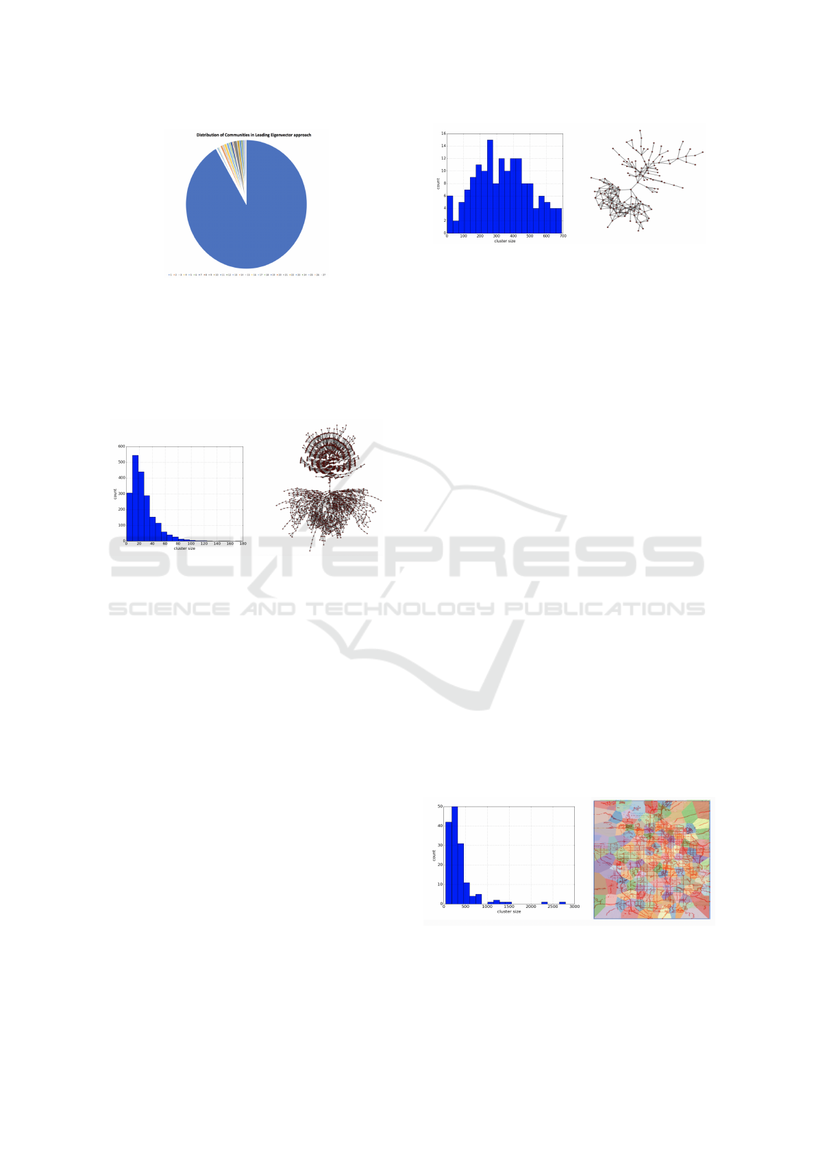
Figure 3: Distribution of communities in Leading Eigen-

vector approach.

nodes of Salt Lake City graph with the distribution as

shown in ﬁgure 4. The distribution looks like a trun-

cated normal distribution, having most of the commu-

nity sizes of the range of 10 to 40 which makes this

approach a good candidate for our case.

Figure 4: Left: Distribution of communities in Label Prop-

agation approach. The dots represent communities.

Multilevel. Multilevel (Yang et al., 2016) approach

proposes a heuristic-based method that is based on

modularity optimization. Based on modularity opti-

mization, a good division of a network into commu-

nities is when the edges inside the group are dense

while the number of edges between groups is signiﬁ-

cantly lower.

The algorithm is divided in two phases that are re-

peated, iteratively. It ﬁrst starts with assigning a dif-

ferent community to each node of the network. Then,

for each node i and its neighbors, the gain of modu-

larity is calculated by removing i from its own com-

munity and by placing it in the community of j. The

node i is then placed in the community for which this

gain is maximum but only if this gain is positive. If

no positive gain is possible, i stays in its original com-

munity. This process is applied repeatedly and se-

quentially for all nodes until no further improvement

can be achieved and the ﬁrst phase is then complete.

It gave us 157 communities on 56753 main nodes of

Salt Lake City (Figure 5).

Figure 5: Left: Distribution of communities in Multilevel

approach. The dots represent communities.

3.5.2 K-means Clustering

Graph clustering is the task of grouping the vertices of

the graph into clusters. Generally, a cluster refers to

a collection of data points aggregated together due to

the certain similarities using unsupervised methods.

There are various clustering methods to be used on

graphs and in this work, we used k-means.

The K-means clustering (Macqueen, 1967) aims

to partition n observations into k clusters in which

each observation belongs to the cluster with the near-

est mean of distance, serving as the centroid of the

cluster. The K-means algorithm starts with a ﬁrst

group of randomly selected centroids, which are used

as the beginning points for every cluster, and then per-

forms iterative calculations to optimize the positions

of the centroids. It ends when there is no change in the

value of centroids or the deﬁned number of iterations

has been achieved.

In K-means, for determining the optimal K (the

number of clusters), we used ’elbow’ method (Mac-

queen, 1967) which ﬁts the model with a range of

values for K and looks at the percentage of variance

inside clusters versus the number of clusters. If the

point of inﬂection on the curve is seen, then it is a

good indication that the underlying model ﬁts best at

that point. After clustering the city graph using k-

means method, the node with highest trafﬁc in that

region is used as exemplar of the nodes in that cluster.

As Figure 6 shows, K-means gives us the total of 151

clusters.

Figure 6: Left: Distribution of main nodes in each cluster of

K-means clustering approach. Right: Visualization of clus-

ters on Salt Lake City. Each color represents one cluster.

Red points represent main ways of the city.

Scalable Stochastic Path Planning under Congestion

459

Figure 7: Left: Distribution of main nodes in each partition.

Right: Visualization of partitions on Salt Lake City. Each

color represents one partition.

3.5.3 Grid based City Partitioning

In this approach, we partition the city based on a sim-

ple gird of 10 * 15 to have 150 partitions. Figure 7

shows the distribution of partitions. Grid based parti-

tioning is used as a baseline in our experiments as it

provides almost an even distribution of nodes in par-

titions.

3.6 Pre-processing: Building Distance

Oracles

Pre-processing helps in quickly ﬁnding paths between

each two nodes and minimizes the time for querying

in a motion planning graph. At each time step of up-

date (which is every week), distance oracles are ex-

ecuted, and the values are used for all types of path

ﬁnding solutions. Given an n-vertex weighted planar

graph G, a distance oracle for G is a data structure that

efﬁciently answers distance queries between pairs of

vertices (u, v) in G. One way is to simply store an

n ×× n-distance matrix for a n-vertex graph. In that

case, each query can be answered in constant time,

but the space requirement is large. Therefore, we are

looking for a solution which answers queries in real

time and efﬁcient in terms of space.

Approximation is a way of making distance or-

acles more compact. Approximate solutions aim to

ﬁnd the solutions which are not exact but clearly

close. Besides, the solution is space and time efﬁ-

cient. Approximation in our model utilizes the exem-

plars and instead of ﬁnding an exact path from source

to destination, it plans a approximate oath through ex-

emplars (details of approach is explained in 3.7).

Distance oracles store the best path for each type

of agent goals between every pair of exemplars for

different time slots of each day of week. In our case,

the whole graph is reduced to exemplars that repre-

sent regions of the graph and we use the path ﬁnding

approach explained in 3.4 to ﬁnd paths between ex-

emplars for each time slot of day/week.

Distance Oracles are updated every week, in or-

der to reﬂect recent trafﬁc patterns on the edges of

Figure 8: Blue circles are exemplars of regions. Green cir-

cles are the typical source and destination.

the city. In every update, data is considered based on

the preceding year data from the date of updating dis-

tance oracle. We store distance oracles for all days of

the week, every 10 minutes time slots and have them

updated weekly. The process of updating distance or-

acles are ofﬂine.

3.7 Scalable Algorithm

When a path ﬁnding request comes, based on the time

of the day, agent’s goal and deadline, source and des-

tination nodes are connected to the respective exem-

plars. Each node has up to nine exemplars around

it, one candidate is the exemplar of the region it is

located and the others are the exemplars of neighbor-

ing regions. Based on the hypothetical direct path be-

tween source and destination, the nodes get connected

to the exemplars with closest similarity to the direc-

tion of that hypothetical path.

For ﬁnding a path that connects source, destina-

tion nodes to their own exemplar, we consider short-

est length path. Then, the best path between the two

exemplars are fetched from the distance oracles and

ﬁnal paths is sent as the result of the query. The path

between exemplars may have other exemplars in the

way, but it does not necessarily need to go through

other exemplars. Figure 8 illustrates the typical path

between source and destination.

4 EXPERIMENTS AND RESULTS

Our experiments are designed to answer the following

questions: 1) how accurate are the approximate paths

in comparison with the exact paths and 2) how much

time we save when we use approximate paths instead

of exact paths.

For the purpose of experiments, we choose 1000

source, destination pairs randomly among all of the

possible source, destination pairs to represent the path

planning universe at different time slots of weekdays

including peak hours and non-peak hours. For each

path planning query, we have the following inputs:

a) source, b) destination, c) time of query, d) dead-

ICAART 2021 - 13th International Conference on Agents and Artiﬁcial Intelligence

460

line and, e) agent’s goal. Then, ﬁrst we ﬁnd the best

path using ’exact’ path planning approach explained

in 3.4 and then using the ’approximate’ path planning

approach explained in 3.7 which works on the set of

exemplars found by a) community detection, b) clus-

tering and c) grid approaches.

4.1 How Many Partitions is Needed?

In picking the right community detection method, the

main consideration is the number of partitions it gen-

erates and the number of nodes the method put in each

partition. Partitioning is mainly used to reduce the

number of nodes in the large scale graph in order to

improve the query time. Obviously, the more the par-

titions the more accurate the results. Hence, we don’t

want to deviate too much from the goal which is sum-

marizing the large scale graph while keeping the ac-

curacy in the acceptable range.

For checking the effect of number of partitions

on accuracy of approximate path planning method,

we use grid-based partitioning as baseline and played

with the number of partitions for one of the agents’

goals. Accuracy of approximate path planning is mea-

sured by its deviation from exact path for each source

and destination for the 1000 samples.

Figure 9 shows the mean difference of travel time

of exact and approximate paths for the agents goal of

highest probability path for the variation of partitions

of the city using grid-based method. As it shows, the

more the partitions the more accurate the paths are.

However, having more partitions increases the node

size which leads in larger distance oracles. Based on

ﬁgure 9, having 150 to 200 partitions looks reason-

able number of partitions with the mean difference of

travel time of exact and approximate paths around 6

percent for peak and non-peak hours.

Figure 9: Number of partitions vs the mean difference of

travel time of exact and approximate path.

Figure 10: Relative difference of mean and variance of

travel time of paths for exact and approximate approach

for peak and non-peak hours for the agent’s goal of high-

est probability path.

4.2 Which Community Detection

Method is Used?

Among the four community detection methods that

we used,’Label propagation’ 3.5.1 and ’Multilevel’

3.5.1 were the two good candidates for our case.

Label propagation partitions Salt Lake City to 2007

communities which most of the communities have

roughly 20 to 40 nodes in them. Multilevel divides

the city to 157 communities and in average each com-

munity includes 200 to 400 nodes in it. For a city

like Salt Lake City, Multi-level provides a good dis-

tribution of clusters, hence we select this approach for

community-based graph partitioning.

4.3 How Accurate Are the Approximate

Paths?

Highest Probability Path. Figure 10 shows the rel-

ative difference of mean and variance of travel time

of paths between exact and approximate path plan-

ning approaches for peak and non-peak hours. As it is

shown, Multi-level community approach is the closest

to exact paths in comparison to clustering (k-means)

and grid-based partitioning. The relative difference

of travel time of all of the approximate approaches is

more signiﬁcant in peak hour in comparison to non-

peak hour. As in non-peak time, the trafﬁc is not high,

both approximate and exact approach are almost the

same. These graphs show that in peak hour, the mean

of travel time of the approximate path using commu-

nity approach is just 8 percent longer than the exact

path and the variance is just 7 percent away.

Figure 11 shows among all of the 1000 source-

destination samples of the experiment, how many

Scalable Stochastic Path Planning under Congestion

461

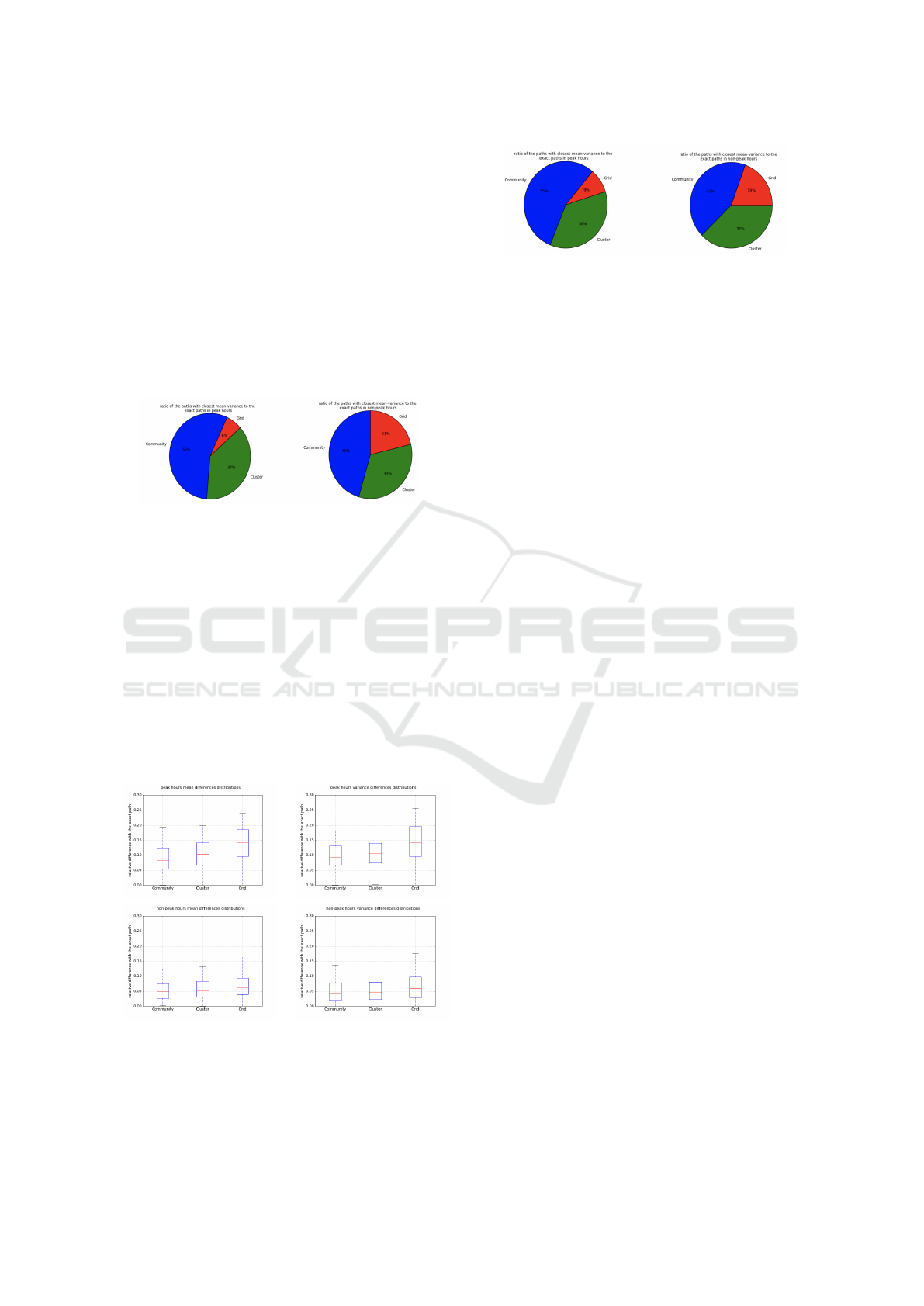
times each of the approximate path planning ap-

proaches (community, cluster and grid) has the clos-

est (mean, variance) of travel time to the exact paths.

Based on ﬁgure 11, in peak hour, 55 percent of the

closest paths to the exact were from community ap-

proach. As it can be seen, in peak hour, most of

the closest paths in both peak and non-peak hour are

found either by community approach or cluster ap-

proach, with some small fraction of grid approach.

While in non-peak hour the ratio is similar for com-

munity, cluster and grid approach. This emphasizes

the fact that, having an accurate graph clustering ap-

proach is crucial in the time of high trafﬁc.

Figure 11: Ratio of paths with the closest mean-variance

to the exact path in peak and non-peak hour for the agent’s

goal of highest probability path.

Shortest Travel Time. Figure 12 and Figure 13 are

the same experiments for the agents that are interested

to select a path with shortest en-route time. Similar

to the previous section, community method has the

closest travel time to the exact path among other ap-

proximate approaches. Approximate path planning

methods in peak hour have larger travel time differ-

ence than non-peak time and in peak time the mean

of community method is 8 percent and its variance is

9 percent away from exact path.

Figure 12: Relative difference of travel time of mean and

variance of paths for exact and approximate approach for

peak and non-peak hours for the agent’s goal of shortest en-

route time.

Figure 13: Ratio of paths with the closest mean-variance to

the exact path for the agent’s goal of shortest en-route time.

4.4 Time and Space Complexity of

Approximate Approaches

As we have seen in the previous experiment, the mean

and variance of approximate approach has the rela-

tive difference of roughly 8 percent to the exact ap-

proach. However, path ﬁnding queries are responded

in real time. In query time, source, destination nodes

get connected to their exemplars and a pre-computed

solution is being fetched from distance oracles.

Now, the question is on the amount of space we

need for storing the approximate paths. In this ap-

proach, we reduce the city graphs by grouping the

similar nodes to each other. For example, the city

graph of Salt Lake City with 56753 nodes and it is

reduced to 157 exemplars. Hence, the nodes in one

community are closely connected to each other and

the approximate algorithm is at least 90 percent good

as the exact approach. For each time slot of day/week,

the best path from the 157 nodes are stored in distance

oracles with respect to the two possible goals of the

system. The rest of the nodes are just connecting to

their exemplars. If we consider nodes of the city as N,

and the number of exemplars as M, instead of storing

N ∗N paths we are storing N ∗M +M ∗M paths which

in our case N is 56753 and M is 157.

5 CONCLUSION AND FUTURE

WORK

In this paper, we proposed a scalable algorithm that

is practical in large scale path planning applications

which suits best for the use cases where agents have

goals, and planner aims to satisﬁes agents’ goals

rather than just providing a path which can move

agents from a source node to a destination node. City

is modelled as a large scale graph and agents have

two types of goals: 1) those who look for the path

with highest probability of reaching destination be-

fore deadline, and 2) the agents who are interested to

have the shortest travel duration while they are ﬂexi-

ble on the time they can leave. Associated with each

path is a deﬁned cost and the goal of the path plan-

ICAART 2021 - 13th International Conference on Agents and Artiﬁcial Intelligence

462

ner is to ﬁnd a path that satisﬁes the agents’ goals

with minimum cost. For expediting the path plan-

ning process, the city is partitioned and each part

is represented with an exemplar. The exemplar of

each partition is the node with the highest trafﬁc on

that region. For partitioning the city graph, we used

three approaches: 1) community detection methods,

2) k-means clustering, and 3) grid based partition-

ing. When a path planning request comes, source

and destination nodes are connected to their corre-

sponding exemplars with respect to the path direc-

tion and the path between exemplars is retrieved. The

paths between exemplars are stored in distance ora-

cles based on the preceding year data at the time of

update and the oracles are updated every week to re-

ﬂect the recent changes on the network. Results show

that among all of the graph clustering approaches,

community-based approaches produce closer results

to exact path planning approach. Approximation pro-

vides paths with mean and variance which are not ex-

act but clearly close to that exact paths, while the so-

lution is space and time efﬁcient.

The main contribution of current work is pro-

viding a paradigm to handle large scale path plan-

ning requests utilizing pre-computation and approx-

imation. Graph partitioning reduces the graph size;

pre-computation helps in answering the queries in

real time and approximation helps in reducing the

space needed for storing the paths ahead of the time.

Even though the approximate paths are not as accu-

rate as exact paths, but they have acceptable accuracy

in comparison to the actual paths given the fact that

they saved a lot of time and space in the whole pro-

cess. Possible future work of this research includes:

a) trying other existing graph clustering methods such

as graph separators, b) adding new agents goals to the

domain and c) considering trafﬁc data prediction to

enhance the decision making process which is cur-

rently based on historical data.

REFERENCES

Ahmadi, K. and Allan, V. H. (2017). Stochastic Path Find-

ing under Congestion. In 2017 International Confer-

ence on Computational Science and Computational

Intelligence (CSCI), pages 135–140.

Bast, H., Funke, S., Sanders, P., and Schultes, D. (2007).

Fast Routing in Road Networks with Transit Nodes.

Science, 316(5824):566–566.

Bauer, R., Columbus, T., Rutter, I., and Wagner, D. (2016).

Search-space size in contraction hierarchies. Theoret-

ical Computer Science, 645.

Edler, D., Guedes, T., Zizka, A., Rosvall, M., and Antonelli,

A. (2017). Infomap Bioregions: Interactive Mapping

of Biogeographical Regions from Species Distribu-

tions. Systematic Biology, 66(2):197–204.

Fan, Y. and Nie, Y. (2006). Optimal Routing for Maximiz-

ing the Travel Time Reliability. Networks and Spatial

Economics, 6(3):333–344.

Frederik Lardinois, Jochen Topf, S. C. (2011). Open-

StreetMap. UIT Cambridge.

Garza, S. E. and Schaeffer, S. E. (2019). Community detec-

tion with the Label Propagation Algorithm: A survey.

Physica A: Statistical Mechanics and its Applications,

534:122058.

Geisberger, R., Sanders, P., Schultes, D., and Vetter, C.

(2012). Exact Routing in Large Road Networks Us-

ing Contraction Hierarchies. Transportation Science,

46(3):388–404.

Gutman, R. (2004). Reach-Based Routing: A New Ap-

proach to Shortest Path Algorithms Optimized for

Road Networks. pages 100–111.

Hart, P. E., Nilsson, N. J., and Raphael, B. (1968). A for-

mal basis for the heuristic determination of minimum

cost paths. IEEE Transactions on Systems Science and

Cybernetics, 4(2):100–107.

Macqueen, J. (1967). Some methods for classiﬁcation and

analysis of multivariate observations. In In 5-th Berke-

ley Symposium on Mathematical Statistics and Prob-

ability, pages 281–297.

Nie, Y. M. and Wu, X. (2009). Shortest path problem con-

sidering on-time arrival probability. Transportation

Research Part B: Methodological, 43(6):597–613.

Niknami, M. and Samaranayake, S. (2016). Tractable

Pathﬁnding for the Stochastic On-Time Arrival Prob-

lem. In Goldberg, A. V. and Kulikov, A. S., editors,

Experimental Algorithms, Lecture Notes in Computer

Science, pages 231–245. Springer International Pub-

lishing.

Nikolova, E. (2010). Approximation algorithms for reli-

able stochastic combinatorial optimization. In Pro-

ceedings of the 13th International Conference on Ap-

proximation, and 14 the International Conference on

Randomization, and Combinatorial Optimization: Al-

gorithms and Techniques, APPROX/RANDOM’10,

page 338–351, Berlin, Heidelberg. Springer-Verlag.

Ruaridh Clark, M. M. (2018). Eigenvector-based commu-

nity detection for identifying information hubs in neu-

ronal networks | bioRxiv.

Rus, S. L. B. K. G. R. M. (2020). Method and apparatus for

trafﬁc-aware stochastic routing and navigation.

Sabran, G., Samaranayake, S., and Bayen, A. (2014). Pre-

computation techniques for the stochastic on-time ar-

rival problem. In Proceedings of the Meeting on Al-

gorithm Engineering & Expermiments, page 138–146,

USA. Society for Industrial and Applied Mathematics.

Samaranayake, S., Blandin, S., and Bayen, A. M. (2012).

Speedup Techniques for the Stochastic on-time Ar-

rival Problem. In ATMOS.

Utah Trafﬁc, . (2020). UDOT: Utah Department of Trans-

portation.

Yang, Z., Algesheimer, R., and Tessone, C. (2016). A

Comparative Analysis of Community Detection Algo-

rithms on Artiﬁcial Networks. Scientiﬁc Reports, 6.

Scalable Stochastic Path Planning under Congestion

463