A Cone Beam Computed Tomography Annotation Tool for Automatic

Detection of the Inferior Alveolar Nerve Canal

Cristian Mercadante

, Marco Cipriano

, Federico Bolelli

, Federico Pollastri

Mattia Di Bartolomeo

, Alexandre Anesi

and Costantino Grana

Department of Engineering “Enzo Ferrari”,

University of Modena and Reggio Emilia, Via P. Vivarelli 10, 41125 Modena, Italy

Surgery, Dentistry, Maternity and Infant Department, Unit of Dentistry and Maxillo-Facial Surgery,

University of Verona, P.le L.A. Scuro 10, 37134 Verona, Italy

Department of Medical and Surgical Sciences for Children & Adults, Cranio-Maxillo-Facial Surgery,

University of Modena and Reggio Emilia, Largo del Pozzo 71, 41124 Modena, Italy

crimerca96@gmail.com, mattiadiba@hotmail.it

Keywords:

CBCT, IAC, IAN, Annotation Tool, Segmentation.

Abstract:

In recent years, deep learning has been employed in several medical ﬁelds, achieving impressive results. Un-

fortunately, these algorithms require a huge amount of annotated data to ensure the correct learning process.

When dealing with medical imaging, collecting and annotating data can be cumbersome and expensive. This

is mainly related to the nature of data, often three-dimensional, and to the need for well-trained expert tech-

nicians. In maxillofacial imagery, recent works have been focused on the detection of the Inferior Alveolar

Nerve (IAN), since its position is of great relevance for avoiding severe injuries during surgery operations

such as third molar extraction or implant installation. In this work, we introduce a novel tool for analyzing

and labeling the alveolar nerve from Cone Beam Computed Tomography (CBCT) 3D volumes.

1 INTRODUCTION

Maxillofacial surgery is a medical-surgical ﬁeld that

concerns the diagnosis and treatment of a wide vari-

ety of head and neck pathologies, including functional

and aesthetic problems. Maxillofacial surgical inter-

ventions comprise oral and dental operations. Among

the cited surgical interventions, the extraction of im-

pacted teeth (especially third molars) and the implant-

prosthetic rehabilitation are two of the most common

procedures. This kind of surgical interventions are

routinely executed and may become very tricky due

to the risk of damaging the Inferior Alveolar Nerve

(IAN).

This sensory nerve supplies the omolateral sensi-

bility to part of the lower third of the face and of the

inferior dental arch. In order to preserve this noble

structure during the surgery, an accurate preoperative

planning must be done and has to include the local-

ization of the IAN. Its position might be indirectly de-

duced via the individuation of the mandibular canal,

also known as Inferior Alveolar Canal (IAC), which

runs inside the mandibular bone. The nerve might be

in close relation to the roots of impacted teeth (es-

Figure 1: 3D view of a jawbone (gray) underlying the lo-

cation of the IAC (red). The original volume has been ac-

quired with Cone Beam Computed Tomography.

pecially the molars) and a detailed 3D description

of their positions must be comprehended before the

surgery. A dental implant consists in the surgical in-

sertion of an artiﬁcial root into the jawbone to provide

anchorage for a dental prosthesis replacing the miss-

ing tooth (implant-prosthetic rehabilitation). To this

purpose, to plan and place accurately a dental implant

it is mandatory to know the linear distance from the

midpoint of the alveolar crest to the IAC.

In order to facilitate the identiﬁcation of the IAN,

many computer-based techniques have been proposed

in the past. Most of the approaches available in the

724

Mercadante, C., Cipriano, M., Bolelli, F., Pollastri, F., Di Bartolomeo, M., Anesi, A. and Grana, C.

A Cone Beam Computed Tomography Annotation Tool for Automatic Detection of the Inferior Alveolar Nerve Canal.

DOI: 10.5220/0010392307240731

In Proceedings of the 16th International Joint Conference on Computer Vision, Imaging and Computer Graphics Theory and Applications (VISIGRAPP 2021) - Volume 4: VISAPP, pages

724-731

ISBN: 978-989-758-488-6

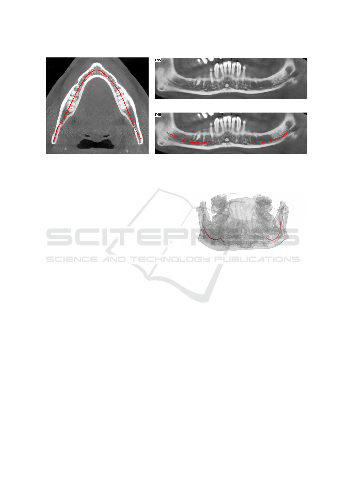
(a) Axial Slice

(b) Original Panoramic View

Figure 2: Example of CT annotation based on 2D panoramic views. (a) is an axial slice of the CT where a panoramic base

curve is highlighted in red. (b) is the panoramic view obtained from the CT-volume displaying voxels of the curved plane

generated by the base curve and orthogonal to the axial view. (c) is the same view of (b) showing a manual annotation of the

IAC performed by an expert technician. A 3D view of the CT scan with the same annotation as (c) is reported in Figure 3.

literature focus on the identiﬁcation of the IAC. As

a matter of fact, the canal is clearly identiﬁable in

both 2D panoramic radiography —also named Or-

thoPantomoGram (OPG)— and Computed Tomogra-

phy (CT) (Sotthivirat and Narkbuakaew, 2006).

Algorithms based on panoramic radiography re-

ported higher accuracy (Vinayahalingam et al., 2019).

However, OPG images just show the IAN from a sin-

gle point of view, masking the real complexity of the

3D canal structure. Moreover, such a kind of images

usually provide geometrical distorted data (Abra-

hams, 2001) and no information about depth (Sot-

thivirat and Narkbuakaew, 2006). This is why state-

of-the-art approaches tackle the task considering the

entire 3D volume obtained with CT scanners (Kondo

et al., 2004; Kwak et al., 2020). These three-

dimensional data can be reformatted into panoramic

reconstructions (panoramic views) thus being able to

apply 2D strategies also on 3D data. With respect to

OPG, panoramic reconstructions are not affected by

distortion, superimposition of other tissues or magni-

ﬁcation errors, permitting a more accurate assessment

of CT data.

In recent years, deep learning algorithms have re-

vealed to be extremely effective solutions to tackle

multiple image processing and computer vision tasks.

In particular, Convolutional Neural Networks (CNNs)

are currently the cornerstone of medical image anal-

ysis (Ronneberger et al., 2015; Esteva et al., 2017;

Canalini et al., 2019; Pollastri et al., 2019; Ligabue

et al., 2020; Pollastri et al., 2021). These techniques

have been recently applied also to the segmentation of

the IAC (Vinayahalingam et al., 2019; Hwang et al.,

2019; Kwak et al., 2020). Unfortunately, they require

Figure 3: 3D view of the manual annotation performed by

an expert technician on the panoramic of Figure 2c.

huge amounts of data, which are hard to obtain and

particularly expensive to annotate, especially in med-

ical ﬁelds. However, simple elements like lines and

colors are learned from the ﬁrst convolutional layers

of CNNs models. For this reason, neural networks

pre-trained with existing collections of natural im-

ages can mitigate the need for large annotated medical

datasets (Deng et al., 2009; Li et al., 2015).

Nevertheless, this approach can not be the panacea

since it may introduce biases towards certain charac-

teristics and features. As an example, CNNs trained

using ImageNet are strongly biased in recognizing

textures rather than shapes (Geirhos et al., 2018).

Several proprietary tools for annotating the infe-

rior alveolar canal from computed tomography scans

are available in the literature. Such tools are usually

supplied together with CT scanners and not other-

wise accessible. Moreover, most of them only pro-

vide two dimensional annotation mechanisms based

on panoramic reconstructions from CT data (an ex-

planatory example is reported in Figure 2).

A Cone Beam Computed Tomography Annotation Tool for Automatic Detection of the Inferior Alveolar Nerve Canal

725

This paper proposes a novel IAC Annotation Tool

(IACAT in short) that aims to overcome the aforemen-

tioned limitations, guaranteeing a more accurate an-

notation while speeding up and simplifying the man-

ual effort of expert technicians.

In Section 2, imaging techniques for maxillofacial

surgery and deep learning approaches for the auto-

matic detection of the inferior alveolar nerve are de-

tailed, focusing on the employed data. Section 3 de-

scribes the annotation tool released with this paper.

Finally, some conclusions are drawn in Section 4.

2 RELATED WORK

2.1 Imaging for Maxillofacial Surgery

Many imaging techniques have been used in the past

for implant dentistry. Among them, OrthoPantomo-

Gram (OPG), Computed Tomography (CT), and Cone

Beam Computed Tomography (CBCT) are certainly

the most widespread. In clinical research, CBCT is

increasingly being used for 3D assessment of bone

and soft tissue (Benic et al., 2015).

The term orthopantomogram, orthopantomogra-

phy, panoramic tomography or OPG in short, refers to

panoramic single image radiography of the mandible,

maxilla and teeth. This technique is based on X-ray

and the OPG unit is designed to rotate around the head

of the patient during the scan. It represents an inex-

pensive and rapid way to evaluate the gross anatomy

of the jaws and related structures, but its limits are

bidimensionality and structure distortion.

Computed Tomography, instead, refers to a com-

puterized X-ray imaging procedure that provides

more complete and detailed information than OPG.

CT employs a narrow beam of X-rays and the ma-

chine emitting this beam quickly rotated around the

body, producing signals that are then processed by a

computer. The output of the CT scanner are cross-

sectional images (slices) of the analyzed body section.

Sequential slices can be digitally stacked to form a 3D

volume, allowing for easier identiﬁcation and location

of basic structures.

Cone Beam Computed Tomography is a variation

of the traditional Computed Tomography and rep-

resents the most commonly employed 3D imaging

modality in dentistry, both for treatment planning and

postoperative evaluation (Jaju and Jaju, 2014).

A CBCT scanner employs a cone beam radiating

from an X-ray source in the shape of a cone. The

use of this particular shape allows to cover large vol-

umes while performing a single rotation around the

patient. CBCT imaging is powerful and presents a de-

creased effective radiation dose exposure to patients

compared to traditional multi-slice CT (Silva et al.,

2008; Ludlow and Ivanovic, 2008; Loubele et al.,

2009; Carraﬁello et al., 2010)

The entire 3D volume is then reconstructed pro-

cessing acquired data with speciﬁc algorithms. A

sample view of CBCT-acquired 3D volume is re-

ported in Figure 1.

2.2 IAC Automatic Detection

Given the relevance of the task, many efforts have

been given to employ computer vision for IAC au-

tomatic detection. The ﬁrst approach (Kondo et al.,

2004) consisted in reformatting the original CT im-

ages to obtain panoramic reconstructions from CT

data (panoramic views), which are a series of cross-

sectional images along the mandible (lower jawbone).

Voxel intensities and 3D gradients are then exploited

to identify empty canals in the panoramic views. The

axis of the IAC is then traced out by a 3D line-tracking

technique, effectively extracting the IAC despite the

open structure of the surrounding bone.

In the same year, Hanssen et al. presented a

method for 3D segmentation of the same nerve chan-

nels in the human mandible. Their technique utilizes

geodesic active surfaces, implemented with level sets,

and consists of two steps. For the ﬁrst step, two points

are deﬁned to denote the entry and exit of the nerve

channel, and a connecting path of minimal action in-

side the channel is calculated. This calculation is

driven by the gray values in proximity to the two de-

ﬁned points inside the channel. For the next step, the

authors exploit this path as an initial conﬁguration,

and let an active surface evolve until the inner borders

of the channel are reached (Hanssen et al., 2004).

Two years later a new technique was introduced

to automatically detect the alveolar nerve canals on

panoramic reconstructions from CT data (Sotthivirat

and Narkbuakaew, 2006). By using a set of axial

CT images acquired from the CT scanner, a series

of panoramic images are generated along the dental

curve. Generated images are then processed by means

of contrast enhancement and Gaussian smoothing ﬁl-

tering before being fed to a detection algorithms

based on the distance transform of the edge image,

morphological operations, and an approximation of

the nerve canals shape.

In more recent times this task has been affected,

as the the rest of the medical imaging area, by

the groundbreaking rise of deep learning. In 2019,

Vinayahalingam et al. focus on detecting the IAN and

the third molar in Orthopantomogram Panoramic Ra-

VISAPP 2021 - 16th International Conference on Computer Vision Theory and Applications

726

(a) Closing & Thresholding (b) CCL (c) Skeletonization (d) Polynomial Approx.

Figure 4: Automatic arch detection steps.

diographs (OPG) (Vinayahalingam et al., 2019).

The authors claim that speciﬁc radiographic fea-

tures on OPGs such as darkening of the root, nar-

rowing of the mandibular canal, interruption of the

white line, are risk factors for IAN injuries. Accord-

ingly, they employ deep learning in the detection of

third molars, mandibular canals, and for the identiﬁ-

cation of certain radiological signs for potential IAN

injuries.

The following year, a preliminary research for a

dental segmentation automation tool on CT scans has

been published (Kwak et al., 2020). In this paper, a set

of experiments were conducted on models based on

2D SegNet (Badrinarayanan et al., 2017), 2D and 3D

U-Net (Ronneberger et al., 2015; C¸ ic¸ek et al., 2016).

3 THE IAC ANNOTATION TOOL

Most of the datasets employed in literature for the au-

tomatic segmentation of the inferior alveolar nerve

have been annotated using proprietary software, e.g.

Photoshop

and Invivo

. However, working with

3D data can be laborious and time-consuming. This

paper proposes a tool for smoothing the burden of

manual annotation, speciﬁcally designed for the IAN

canal. It processes and visualizes CBCT data stored

in DICOM format, driving the user towards the anno-

tation of axial images, panoramic and cross-sectional

views. Annotated data can be easily exported to be

employed in multiple tasks, e.g. the training of deep

learning models.

3.1 Pre-processing

The tool requires a DICOM input, in particular a

DICOMDIR ﬁle linked to dcm ﬁles, representing single

axial images of the scan. Radiography values repre-

sent attenuation of the X-rays emitted and captured

by a detector. These measures are always considered

https://www.photoshop.com

https://www.anatomage.com/invivo

on the Hounsﬁeld scale, where higher numbers indi-

cate a high attenuation. After loading the scan vol-

ume, a saturation threshold is applied: bone voxels

have Hounsﬁeld units usually in the range [400, 3000]

(Nysj

o, 2016), but peak values around 14 000 usually

correspond to the tooth crown and enamel (less of 2%

of the volume). Since the IAN canal is not involved in

this operation, it is reasonable to saturate from the top

with the 0.98 percentile value. The values are then

normalized in the range [0, 1] and stored as 32 bits

ﬂoating point values without loosing any information.

This pre-processing acts as a contrast stretching of the

original DICOM values.

3.2 Axial Image Annotation

After loading the input data, the arch approximation

that better describes the canal course must be iden-

tiﬁed inside one of the axial images. This process

is partially automated and aims to segment the gums

region in order to obtain a skeleton and to approxi-

mate it with a polynomial. A morphological closing

(Gil and Kimmel, 2002) with an elliptical 5 × 5 struc-

turing element is applied in order to close gaps in-

side foreground regions. Then, the image is binarized

by selecting the threshold value so that foreground

pixels are between 12% to 16% of the image. Con-

nected Components Labeling (CCL) (Bolelli et al.,

2019) is employed to keep only the biggest object —

the gums— by removing all the other components.

Inner holes are ﬁlled with a second CCL pass, produc-

ing a binary image with the gums region appearing as

a ﬁlled arch. Image skeletonization is then performed

using thinning (Bolelli and Grana, 2019). The out-

put is a one pixel thick curve crossing the dental arch,

which is approximated with a polynomial. The entire

process is depicted in Figure 4.

Once the axial image and its arch approxima-

tion are selected, the tool generates a Catmull-Rom

spline (Catmull and Rom, 1974; Barry and Goldman,

1988) by sampling the polynomial to select the con-

trol points of the spline. This curve is the base of

a Curved Planar Reformation (CPR) that produces

A Cone Beam Computed Tomography Annotation Tool for Automatic Detection of the Inferior Alveolar Nerve Canal

727

(a) (b) (c) (d) (e)

(f) (g) (h) (i) (j)

Figure 5: Morphological Geodesic Active Contours evolution on a sequence of cross-sectional images.

a panoramic 2D image. This view is obtained dis-

playing voxels of the curved plane corresponding the

base curve and orthogonal to the axial slice. When

the user moves, creates or removes control points, the

panoramic view changes accordingly. The goal of this

step is to highlight the IAC on the panoramic view, by

ﬁnding the best arch curve. The user can also offset

the position of this curve in order to produce an upper

and lower panoramic view, thus ensuring a better edit-

ing of the spline itself (Sotthivirat and Narkbuakaew,

2006).

Two offset curves (outer and inner) are drawn with

distance 50 pixels from the main arch. For each

point of the spline, a perpendicular line called Cross-

Sectional Line (CSL) is computed. Since the points

of the spline are as many as the euclidean distance be-

tween two control points, a different resolution of the

spline would generate more or less CSLs. These lines

are the base of Multi Planar Reformations (MPRs)

called Cross-Sectional Views (CSVs). These are 2D

images obtained interpolating the values of the re-

spective base line across the whole volume height.

3.3 Annotating Cross-sectional Views

For each CSV, the user can draw a closed Catmull-

Rom spline to annotate the position of the IAC.

As usual, control points can be created, deleted, or

moved. To speed-up the annotation phase, an active

contour model (Kass et al., 1988) is used to automat-

ically propagate the annotation to the following im-

age. In particular, Morphological Geodesic Active

Contours have been selected (Caselles et al., 1997;

Alvarez et al., 2010): this technique employs mor-

phological operators to evolve the curve, combined

with the concept of energy minimization in the prob-

lem of geodesic curve computation. In absence of

gradients, this algorithm forces the contour to expand

—the balloon factor— whereas other active contour

approaches shrink object shapes.

In order to propagate the annotation to the fol-

lowing (or previous) cross-sectional view, the Mor-

phological Geodesic Active Contours algorithm re-

quires two inputs: the current annotation as a binary

mask, and the gradients of the following (or previous)

CSV. The output of the algorithm is a new annotation

mask from which the tool generates the spline with

an amount of control points that depends on its length

(the longer it is, the more control points are needed

to approximate the real shape). The model runs for 5

iterations, with a smoothing factor of 1, and a balloon

factor of 1. Figure 5 shows the evolution of the spline

in subsequent images, starting from a manual annota-

tion, up to the ninth following image. The model is

able to create accurate annotations without user inter-

vention for many consecutive images. In this exam-

ple, the ﬁrst mistake appears in Figure 5i (the top edge

of the spline), and is propagated into Figure 5j.

Any user adjustment can be automatically propa-

gated to the following views.

The splines are saved as the coordinates of their

control points, and a label mask is generated for each

CSV. The labels employed are four (C¸ ic¸ek et al.,

2016): unlabeled, background, contour, interior. Im-

ages that are not annotated inherit unlabeled class by

default. Otherwise, the mask is set to background,

with the spline labeled as contour and internal pixels

labeled as interior.

3.4 Tilted Cross-sectional Views

An important feature introduced in the IACAT tool

is the extraction of CSVs orthogonal to the canal

slope. To achieve this goal, the Cross-Sectional

VISAPP 2021 - 16th International Conference on Computer Vision Theory and Applications

728

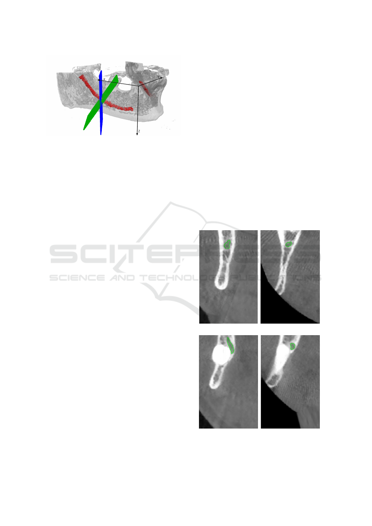
Figure 6: A visualization of the cross-sectional plane ro-

tation around the y axis, as described in Section 3.4. The

original plane is presented in blue, whereas the tilted one is

green. The IAC is red.

Planes (CSPs) used for generating the CSVs are tilted

accordingly.

On the panoramic view, the user can draw two

Catmull-Rom splines which indicate the canal posi-

tion, one for each branch. For each point p of the

spline, the slope can be computed by using the deriva-

tive of a 12

order polynomial ﬁt f :

β(p) = −arctan( f

(p)) (1)

Given the slope of the canal, the cross-sectional

view orthogonal to the canal is obtained as follows:

• The cross-sectional plane is translated so that its

center is placed at the origin of the reference sys-

tem;

• The plane is rotated around the z axis, until it be-

comes parallel to the y axis. The following Equa-

tion shows the rotation matrix, where u is the unit

vector of the plane:





−u

0 0 1





(2)

• The plane is then rotated around the y axis, by the

angle β obtained with Equation 1, using the fol-

lowing rotation matrix:





cosβ 0 sin β

0 1 0

sinβ 0 cosβ





(3)

• Finally, the plane is rotated back around the z axis

to its original position, using the rotation matrix in

Equation 4, and the initial translation is reversed.





−u

0 0 1





(4)

The CSVs are generated from the rotated planes, us-

ing bilinear interpolation. In most cases, since the

canal has a slight inclination, the tilted cross-sectional

views do not differ much from the straight ones. Fig-

ure 7 shows two examples in which tilted views pro-

vide strong improvements to the IAC localization.

3.5 Annotation Re-projection

The re-projection of the labeled masks in 3D is re-

quired to generate the ﬁnal segmentation. A plane

corresponds to each cross-sectional image, which

contains the ﬂoating point coordinates of the volume

voxels used to interpolate a certain pixel in the image.

For each pixel of the image, its label is re-projected in

the corresponding voxel coordinate. To prevent alias-

ing due to the undersampling of the voxel coordinates

in the volume, each label is copied to the positions

corresponding to the f loor and ceil of each coordi-

nate of the plane. Figure 8 shows the results obtained

re-projecting straight cross-sectional images annota-

tion masks in 3D (considering only contour and inte-

rior labels).

The surface of the reconstructed volume is often

irregular, due to the nature of the 2D annotations.

(a) (b)

Figure 7: Comparison of straight (a), (c) and tilted (b), (d)

cross-sectional images.

A Cone Beam Computed Tomography Annotation Tool for Automatic Detection of the Inferior Alveolar Nerve Canal

729

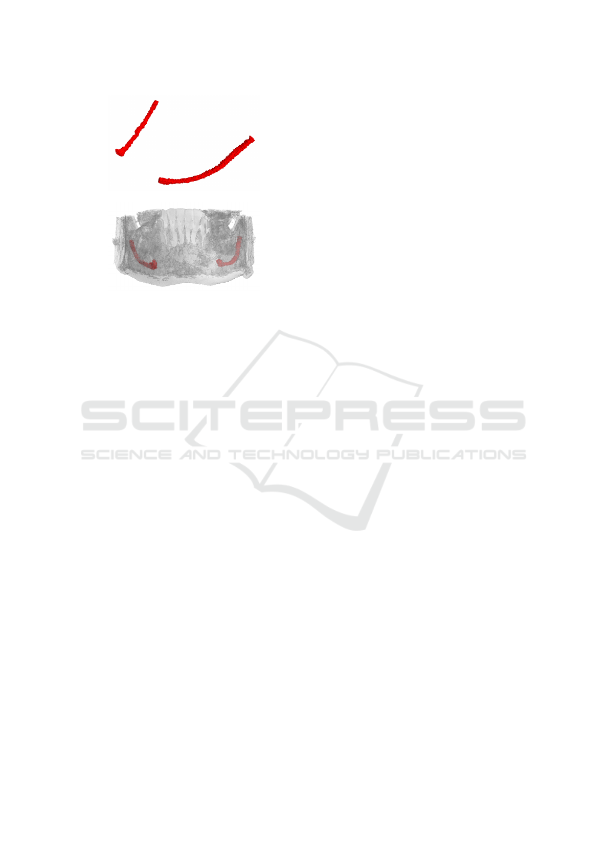
(a)

(b)

Figure 8: (a) 3D view of the canal reconstruction and (b) its

location inside the jawbone.

Therefore, a smoothing process is proposed to pro-

duce a polished contour on the 3D canal shape. A

22 × 22 × 22 kernel is moved with stride 18 along the

reconstructed canal volume. At each step, the convex

hull is evaluated on the current block, obtaining a set

of triangles that composes the convex hull. These tri-

angles are then voxelized and the smoothed canal is

created. The described approach generate a more reg-

ular and uniform segmentation at the expense of the

ﬁnal accuracy.

3.6 Exports

The annotation can ﬁnally be exported as binary npy

ﬁles. The two main formats are the concatenation

of cross-sectional image masks and the re-projected

3D annotation. The tool is also able to generate png

images, both for cross-sectional images and their la-

beled masks, and to create a new DICOM ﬁle with an-

notations as overlays. An important feature of the

tool is the recording of user actions, in particular of

every interaction with the splines (on axial images,

panoramic views and cross-sectional images). In-

deed, future research directions include the automa-

tion of more steps in the annotation process, by learn-

ing from the actions of an expert. Therefore, cre-

ation, removal and changes in splines control points

are recorded, with contextual information, such as the

current cross-sectional image index. Moreover, the

tool records whether the user is propagating the anno-

tations or resetting the current spline. The history of

actions can be saved on disk in json format.

4 CONCLUSION

In this paper we presented IACAT, a software for the

annotation of CBCT scans. The proposed tool com-

prises and improves the functionality of existing an-

notation tools for the segmentation of Inferior Alve-

olar Nerve, simplifying and improving the work of

expert technicians. The image processing techniques

implemented allow to automatically extend manual

annotations carried out on portions of the volume,

thus speeding up the entire process.

REFERENCES

Abrahams, J. J. (2001). Dental ct imaging: A look at the

jaw. Radiology, 219(2):334–345.

Alvarez, L., Baumela, L., Henriquez, P., and Marquez-

Neila, P. (2010). Morphological snakes. In 2010

IEEE Computer Society Conference on Computer Vi-

sion and Pattern Recognition, pages 2197–2202.

Badrinarayanan, V., Kendall, A., and Cipolla, R. (2017).

SegNet: A Deep Convolutional Encoder-Decoder Ar-

chitecture for Image Segmentation. IEEE Transac-

tions on Pattern Analysis and Machine Intelligence,

39:2481–2495.

Barry, P. and Goldman, R. (1988). A Recursive Evaluation

Algorithm for a Class of Catmull-Rom Splines. ACM

SIGGRAPH Computer Graphics, 22:199–204.

Benic, G. I., Elmasry, M., and H

ammerle, C. H. (2015).

Novel digital imaging techniques to assess the out-

come in oral rehabilitation with dental implants: a

narrative review. Clinical Oral Implants Research,

26:86–96.

Bolelli, F., Allegretti, S., Baraldi, L., and Grana, C. (2019).

Spaghetti Labeling: Directed Acyclic Graphs for

Block-Based Connected Components Labeling. IEEE

Transactions on Image Processing, 29(1):1999–2012.

Bolelli, F. and Grana, C. (2019). Improving the Perfor-

mance of Thinning Algorithms with Directed Rooted

Acyclic Graphs. In Image Analysis and Processing -

ICIAP 2019, volume 11752, pages 148–158. Springer.

Canalini, L., Pollastri, F., Bolelli, F., Cancilla, M., Alle-

gretti, S., and Grana, C. (2019). Skin Lesion Segmen-

tation Ensemble with Diverse Training Strategies. In

Computer Analysis of Images and Patterns, volume

11678, pages 89–101. Springer.

Carraﬁello, G., Dizonno, M., Colli, V., Strocchi, S., Taubert,

S. P., Leonardi, A., Giorgianni, A., Barresi, M., Mac-

chi, A., Bracchi, E., et al. (2010). Comparative

study of jaws with multislice computed tomography

and cone-beam computed tomography. La radiologia

medica, 115(4):600–611.

Caselles, V., Kimmel, R., and Sapiro, G. (1997). Geodesic

Active Contours. International Journal of Computer

Vision, 22:61–79.

Catmull, E. and Rom, R. (1974). A Class of Local Interpo-

lating Splines. Computer Aided Geometric Design -

CAGD, 74:317–326.

VISAPP 2021 - 16th International Conference on Computer Vision Theory and Applications

730

C¸ ic¸ek, O., Abdulkadir, A., Lienkamp, S., Brox, T., and Ron-

neberger, O. (2016). 3D U-Net: Learning Dense Vol-

umetric Segmentation from Sparse Annotation. In In-

ternational Conference on Medical Image Computing

and Computer-Assisted Intervention, pages 424–432.

Deng, J., Dong, W., Socher, R., Li, L.-J., Li, K., and Fei-

Fei, L. (2009). ImageNet: A Large-Scale Hierarchical

Image Database. In 2009 IEEE Conference on Com-

puter Vision and Pattern Recognition, pages 248–255.

IEEE.

Esteva, A., Kuprel, B., Novoa, R. A., Ko, J., Swetter, S. M.,

Blau, H. M., and Thrun, S. (2017). Dermatologist-

level classiﬁcation of skin cancer with deep neural net-

works. Nature, 542(7639):115–118.

Geirhos, R., Rubisch, P., Michaelis, C., Bethge, M., Wich-

mann, F. A., and Brendel, W. (2018). ImageNet-

trained CNNs are biased towards texture; increasing

shape bias improves accuracy and robustness. arXiv

preprint arXiv:1811.12231.

Gil, J. Y. and Kimmel, R. (2002). Efﬁcient Dilation, Ero-

sion, Opening,and Closing Algorithms. IEEE Trans-

actions on Pattern Analysis and Machine Intelligence,

24(12):1606–1617.

Hanssen, N., Burgielski, Z., Jansen, T., Lievin, M., Ritter,

L., von Rymon-Lipinski, B., and Keeve, E. (2004).

Nerves-level sets for interactive 3d segmentation of

nerve channels. In 2004 2nd IEEE International

Symposium on Biomedical Imaging: Nano to Macro

(IEEE Cat No. 04EX821), volume 1, pages 201–204.

Hwang, J.-J., Jung, Y.-H., Cho, B.-H., and Heo, M.-S.

(2019). An overview of deep learning in the ﬁeld of

dentistry. Imaging science in dentistry, 49(1):1–7.

Jaju, P. P. and Jaju, S. P. (2014). Clinical utility of dental

cone-beam computed tomography: current perspec-

tives. Clinical, cosmetic and investigational dentistry,

6:29.

Kass, M., Witkin, A., and Terzopoulos, D. (1988). Snakes:

Active contour models. International Journal of Com-

puter Vision, 1(4):321–331.

Kondo, T., Ong, S., and Foong, K. W. (2004). Computer-

based extraction of the inferior alveolar nerve canal

in 3-D space. Computer Methods and Programs in

Biomedicine, 76(3):181–191.

Kwak, H., Kwak, E.-J., Song, J.-M., Park, H., Jung, Y.-H.,

Cho, B.-H., Hui, P., and Hwang, J. (2020). Automatic

mandibular canal detection using a deep convolutional

neural network. Scientiﬁc Reports, 10.

Li, Y., Yosinski, J., Clune, J., Lipson, H., and Hopcroft, J. E.

(2015). Convergent Learning: Do different neural net-

works learn the same representations? In Proceed-

ings of the 1st International Workshop on Feature Ex-

traction: Modern Questions and Challenges at NIPS

2015, pages 196–212.

Ligabue, G., Pollastri, F., Fontana, F., Leonelli, M., Furci,

L., Giovanella, S., Alfano, G., Cappelli, G., Testa, F.,

Bolelli, F., Grana, C., and Magistroni, R. (2020). Eval-

uation of the Classiﬁcation Accuracy of the Kidney

Biopsy Direct Immunoﬂuorescence through Convolu-

tional Neural Networks. Clinical Journal of the Amer-

ican Society of Nephrology, 15(10):1445–1454.

Loubele, M., Bogaerts, R., Van Dijck, E., Pauwels, R., Van-

heusden, S., Suetens, P., Marchal, G., Sanderink, G.,

and Jacobs, R. (2009). Comparison between effec-

tive radiation dose of CBCT and MSCT scanners for

dentomaxillofacial applications. European Journal of

Radiology, 71(3):461–468.

Ludlow, J. B. and Ivanovic, M. (2008). Comparative

dosimetry of dental CBCT devices and 64-slice CT for

oral and maxillofacial radiology. Oral Surgery, Oral

Medicine, Oral Pathology, Oral Radiology, and En-

dodontology, 106(1):106–114.

Nysj

o, J. (2016). Interactive 3D Image Analysis for Cranio-

Maxillofacial Surgery Planning and Orthopedic Ap-

plications. PhD thesis, Uppsala University.

Pollastri, F., Bolelli, F., Paredes, R., and Grana, C. (2019).

Augmenting Data with GANs to Segment Melanoma

Skin Lesions. Multimedia Tools and Applications

Journal, 79(21-22):15575–15592.

Pollastri, F., Maro

nas, J., Bolelli, F., Ligabue, G., Pare-

des, R., Magistroni, R., and Grana, C. (2021). Conﬁ-

dence Calibration for Deep Renal Biopsy Immunoﬂu-

orescence Image Classiﬁcation. In 2020 25th Interna-

tional Conference on Pattern Recognition (ICPR).

Ronneberger, O., Fischer, P., and Brox, T. (2015). U-Net:

Convolutional Networks for Biomedical Image Seg-

mentation. LNCS, 9351:234–241.

Silva, M. A. G., Wolf, U., Heinicke, F., Bumann, A., Visser,

H., and Hirsch, E. (2008). Cone-beam computed to-

mography for routine orthodontic treatment planning:

a radiation dose evaluation. American Journal of Or-

thodontics and Dentofacial Orthopedics, 133(5):640–

e1.

Sotthivirat, S. and Narkbuakaew, W. (2006). Automatic De-

tection of Inferior Alveolar Nerve Canals on CT Im-

ages. In 2006 IEEE Biomedical Circuits and Systems

Conference, pages 142–145.

Vinayahalingam, S., Xi, T., Berge, S., Maal, T., and

De Jong, G. (2019). Automated detection of third mo-

lars and mandibular nerve by deep learning. Scientiﬁc

Reports, 9.

A Cone Beam Computed Tomography Annotation Tool for Automatic Detection of the Inferior Alveolar Nerve Canal

731