
Exploring Slow Feature Analysis for Extracting Generative
Latent Factors
Max Menne
a
, Merlin Sch
¨
uler
b
and Laurenz Wiskott
c
Institute for Neural Computation, Ruhr University Bochum, Universit
¨
atsstraße 150, 44801 Bochum, Germany
Keywords:
Slow Feature Analysis, Representation Learning, Generative Models.
Abstract:
In this work, we explore generative models based on temporally coherent representations. For this, we incor-
porate Slow Feature Analysis (SFA) into the encoder of a typical autoencoder architecture. We show that the
latent factors extracted by SFA, while allowing for meaningful reconstruction, also result in a well-structured,
continuous and complete latent space – favorable properties for generative tasks. To complete the generative
model for single samples, we demonstrate the construction of suitable prior distributions based on inherent
characteristics of slow features. The efficacy of this method is illustrated on a variant of the Moving MNIST
dataset with increased number of generation parameters. By the use of a forecasting model in latent space, we
find that the learned representations are also suitable for the generation of image sequences.
1 INTRODUCTION
Recently, deep generative models have yielded im-
pressive results in the artificial generation of real-
istic high-dimensional image (Karras et al., 2018;
Kingma et al., 2016; Van den Oord et al., 2016b), au-
dio (Van den Oord et al., 2016a; Mehri et al., 2016)
and video (Denton and Fergus, 2018; Tulyakov et al.,
2018) data. At the same time, unsupervised represen-
tation learning has been known to aid effective learn-
ing in goal-oriented frameworks such as reinforce-
ment learning (Sutton and Barto, 2018) or supervised
learning (Goodfellow et al., 2016) when rewards or
labels are sparse. While the use of generative factors
as effective representations in goal-directed learning
is a strong focus of current research (Yarats et al.,
2019; Hafner et al., 2020), the back-direction less so.
To enable unsupervised training of generative
models usually a maximum-likelihood criterion and
the reconstruction error are used in combination as an
optimization objective (Kingma and Welling, 2019).
The majority of realizations of generative models for
complex and high-dimensional data are based either
on the Variational Autoencoder (VAE) (Kingma and
Welling, 2013) or Generative Adversarial Networks
(GANs) (Goodfellow et al., 2014).
a
https://orcid.org/0000-0002-0808-497X
b
https://orcid.org/0000-0002-9809-541X
c
https://orcid.org/0000-0001-6237-740X
We explore a new class of generative models that
is optimized using the principle of temporal coher-
ence in combination with the reconstruction error.
The latter is realized by using an autoencoder archi-
tecture and reconstruction loss, while the former is
realized by Slow Feature Analysis (SFA). In contrast
to the strict end-to-end training procedure of VAEs
and GANs, this allows for principle-based extraction
and subsequent processing of latent factors for gener-
ative purposes, offering separated and more detailed
analyses. SFA uses the principle of slowness as a
proxy for the extraction of low-dimensional descrip-
tive representation from, possibly high-dimensional,
time-series data or data for which other pairwise sim-
ilarities can be defined. In our models, these ob-
tained low-dimensional representations are consid-
ered as latent factors, since they often encode the
elementary properties of the data-generation process
(Franzius et al., 2007; Franzius et al., 2011; Sch
¨
uler
et al., 2019). First theoretical considerations for mod-
elling slow features as generative latent factors have
already been introduced in (Turner and Sahani, 2007),
but are restricted to the linear case. In contrast, our
models are based on non-linear PowerSFA (Sch
¨
uler
et al., 2019). Its applicability to any differentiable
encoder/decoder allows for significantly more pow-
erful encoding and efficient processing of complex
and possibly high-dimensional data, while it can be
trained end-to-end with respect to different objective
functions.
120
Menne, M., Schüler, M. and Wiskott, L.
Exploring Slow Feature Analysis for Extracting Generative Latent Factors.
DOI: 10.5220/0010391401200131
In Proceedings of the 10th International Conference on Pattern Recognition Applications and Methods (ICPRAM 2021), pages 120-131
ISBN: 978-989-758-486-2
Copyright
c
2021 by SCITEPRESS – Science and Technology Publications, Lda. All rights reserved

We start by introducing SFA in Section 2. The ex-
periments presented in Section 3 are based on differ-
ent models and datasets, consisting of synthetic image
sequences, described in Section 3.1 and 3.2. Our anal-
yses focus, in particular, on the latent factors. We in-
vestigate the relationship between their slowness and
reconstructability in Section 3.3 as well as the struc-
ture and properties of the resulting latent space for
generative purposes in Section 3.4. Based on these
findings, we propose a method for the construction of
a prior distribution over the latent factors in Section
3.5. We show that samples from this prior distribu-
tion are suitable for the generation of new images us-
ing the aforementioned decoder. Finally, we extend
one of our models by a forward predictor over the ex-
tracted representation and demonstrate the generation
of image sequences. In Section 4, we discuss our re-
sults and give future directions.
2 SLOW FEATURE ANALYSIS
SFA is an unsupervised learning algorithm which
utilizes the principle of slowness to extract low-
dimensional data-generating factors. The principle of
slowness states that high-dimensional data streams,
which change rapidly over time, are generated by a
small number of comparatively slowly varying fac-
tors.
SFA therefore solves the optimization problem of
the extraction of slow, meaningful features: Given a
time series {x
t
}
t=0,1,...,N−1
consisting of data points
x
t
∈ R
d
, find a continuous input-output function g :
R
d
→ R
e
so that
min
g
hkg(x
t+1
) − g(x
t
)k
2
i
t
(1a)
s.t. hg(x
t
)i
t
= 0
0
0, (1b)
hg(x
t
)g(x
t
)
T
i
t
= I
e
. (1c)
In this context the time average is denoted by h·i
t
and
I
e
refers to the e-dimensional unit matrix. To ensure
an ordering from the slowest to the fastest varying fea-
ture, the following constraint can be additionally ap-
plied for i < j:
∆(g
i
) = hkg
i
(x
t+1
) − g
i
(x
t
)k
2
i
t
≤ hkg
j
(x
t+1
) − g
j
(x
t
)k
2
i
t
= ∆(g
j
).
(2)
These constraints ensure unique (zero mean, equation
(1b)), non-trivial and informative (unit variance and
decorrelation, equation (1c)) solutions.
In the past several different variants (B
¨
ohmer
et al., 2011; Franzius et al., 2007; Escalante-B and
Wiskott, 2020) of the original SFA algorithm (Wiskott
and Sejnowski, 2002) have been proposed to over-
come limitations and improve the performance of
SFA.
A recently introduced version of the SFA algo-
rithm is the so-called Power Slow Feature Analysis
(PowerSFA) (Sch
¨
uler et al., 2019), which is based
on differentiable approximated whitening. This al-
lows the combination of the SFA optimization prob-
lem with differentiable architectures, such as neural
networks, and the optimization in form of a gradient-
based end-to-end training procedure.
One of the main steps in the SFA algorithm is the
whitening of the data which is essential to fulfill the
SFA constraints (equations (1b) and (1c)). The cen-
tral idea of PowerSFA consists of whitening the data
within a differentiable whitening layer. This whiten-
ing layer can be applied to any differentiable archi-
tecture that is used as a function approximator and
ensures that the outputs met the SFA constraints.
Mathematically, PowerSFA can be formalized as
follows: Given a dataset X = [x
0
, x
1
, . . . , x
N−1
] ∈
R
d×N
the output Y ∈ R
e×N
, which approximately
matches the SFA constraints, is calculated by
Y = W (H) with H = ˜g
θ
θ
θ
(X).
The approximated whitening by means of the whiten-
ing layer is described by W : R
N×e
→ R
N×e
and a dif-
ferentiable function approximator, like a neural net-
work, parameterized by θ
θ
θ with ˜g
θ
θ
θ
: R
d
→ R
e
. For op-
timization with respect to the slowness principle, an
error measurement based on a general differentiable
loss function such as
L(S , Y) =
1
N
∑
i
∑
j
s
i j
ky
i
− y
j
k
2
(3)
can be used. In this case s
i j
describes the similarity
between two data points x
i
and x
j
.
3 EXPERIMENTS
In this paper, we focus on the question if generative
latent factors can be extracted using SFA. The central
approach for the development and analysis of a gen-
erative model is based on the embedding of SFA into
the structure of an autoencoder. From this idea, we
derive two main models, which build – in combina-
tion with different datasets based on image sequences
– the foundation for the experiments. The analyses
are divided into the following three key aspects:
Reconstructability. We analyze the recon-
structability of the input data based on the extracted
features and investigate how the SFA constraints
influence the reconstructions.
Exploring Slow Feature Analysis for Extracting Generative Latent Factors
121

Structure of the Latent Space. We explore if the
latent space defined by the extracted latent factors
is structured in a continuous and organized manner,
which is therefore suitable for generative purposes.
Further, the complexity and possible dependencies
between individual factors are considered.
Prior Distribution Over Latent Factors. We try to
manually construct meaningful underlying prior dis-
tributions and check whether samples of these distri-
butions can be decoded in a meaningful way to gen-
erate new data.
3.1 Models
We start by introducing the central models, which
share the same general architecture consisting of a
neural encoder and decoder network. All models
are trained with the ADAM optimization algorithm
(Kingma and Ba, 2014) with Nesterov-accelerated
momentum (Dozat, 2015).
3.1.1 Encoder-Decoder Model
The Encoder-Decoder model consists of an encoder
and decoder network. The encoder is a simple neural
network followed by the PowerWhitening layer of the
PowerSFA framework and embeds the input data into
the latent space. The input layer of the encoder takes a
single 64×64 pixel greyscale image. After flattening,
the resulting 4096-dimensional vector is reduced to
the dimensionality of the latent space by a dense layer.
The output of the dense layer is finally whitened by
the subsequent PowerWhitening layer, which simul-
taneously represents the output layer of the encoder
and outputs the latent factors. The decoder network
consists of a fully-connected feedforward neural net-
work. The decoder receives the latent factors as input
and processes them by a block of five dense layers.
These layers consist of 64, 128, 256, 512 and 4096
units and therefore upsample the activations back to a
4096-dimensional vector or respectively after reshap-
ing to a 64×64 pixel greyscale output image. The
units in the first four dense layers are implemented by
Rectified Linear Units (ReLUs), while for the activa-
tion of the units in the fifth layer a Sigmoid activation
function is used. A visualization of the encoder and
decoder network is provided in Appendix A.
The training procedure of the Encoder-Decoder
model is divided into two steps. First, we train the en-
coder with respect to the general slowness objective
of the PowerSFA framework, introduced in equation
(3) and denoted in the following as L
SFA
(S , Y). In a
second phase the decoder network is optimized with
respect to the cross-entropy loss L
CE
(X,
˜
X) between
the original input images X and the computed output
images
˜
X.
Due to the division of the training process, the de-
coder does not influence the encoder and an unim-
paired learning of a function for the extraction of
slowly varying features by the encoder is guaranteed.
3.1.2 Slowness-Regularized Autoencoder Model
The Slowness-Regularized Autoencoder (SRAE)
model is very similar to the Encoder-Decoder model,
but has the difference that the encoder and decoder
are combined into an autoencoder. We omit the input
layer of the decoder and append the remaining layers
directly to the former output layer of the encoder.
The SRAE model is optimized in an end-to-end
fashion with respect to a composite loss function. It
consists of the sum of the previously introduced cross-
entropy loss L
CE
(X,
˜
X) and the general slowness ob-
jective L
SFA
(S , Y), which is additionally weighted by
a weighting factor α:
L
SRAE
(X,
˜
X, S , Y) = L
CE
(X,
˜
X)+α·L
SFA
(S , Y) (4)
The calculated error is back-propagated through
the entire architecture. The reconstruction error af-
fects thus not only the decoder and its parameters but
also the encoder, its parameters and consequently the
encoding.
By choosing the hyperparameter α = 0, the SRAE
model represents an autoencoder with whitened la-
tent variables, but without regularization within the
loss function. We use this specific configuration as
a baseline. In contrast, for large values of α, a link
to the previously introduced Encoder-Decoder model
is established in the limiting case, as the reconstruc-
tion objective has almost no influence in relation to
the slowness objective anymore.
3.2 Datasets
We evaluate our models on synthetic image data with
different generating attributes. Using affine trans-
formations like translation, rotation or scaling, im-
age sequences with images of the dimension 64×64
are generated from single 28×28 pixel images of the
MNIST (LeCun et al., 2010) dataset. This dataset
generation therefore combines the transformations
used in the affNIST dataset (Tieleman, 2013) with
the idea to generate not only single images but im-
age sequences as in the Moving MNIST (MMNIST)
(Srivastava et al., 2015) dataset. This results in an
extended version of the MMNIST dataset with addi-
tional possible transformations besides the translation
of a digit.
ICPRAM 2021 - 10th International Conference on Pattern Recognition Applications and Methods
122
The datasets can be divided into two classes. The
first class is formed by the so-called moving se-
quences with the defining property of variation in po-
sition. In this case, an image sequence is build by
moving a single digit in the 64×64 frame on linear
trajectories which are reflected at the edges. As an al-
ternative to the variation of the identity of the used
digit, further, a rotation or scaling of the digit can
be applied in conjunction with the variation in posi-
tion. The second class is based on so-called static se-
quences in which the position of the digit is fixed in
the center of the 64×64 pixel image. For this class of
datasets, we vary the identity and rotation or scaling
of the digit.
Besides the image sequences, each dataset is aug-
mented by a similarity matrix S , which defines the
similarity between all images. To extract slowly vary-
ing features, the similarity is based on the temporal
proximity, which can be expressed by the Kronecker
delta s
i j
= δ
i, j+1
leading to a connection between con-
secutive images. Alternatively, the similarity matrix
can define a more general neighborhood-based rela-
tionship based on certain attributes of the individual
images like position or identity of the digit. This al-
lows an optimization with respect to a graph-based
embedding.
This dataset generation enables the construction of
arbitrarily large and complex datasets as well as a pre-
cise control over the data-generating attributes. These
properties facilitate the exploration and analysis of the
extracted latent factors.
3.3 Slowness versus Reconstructability
In this section, we investigate the relationship be-
tween the principle of slowness and the recon-
structability based on the extracted latent features.
The experiment examines whether these two princi-
ples work in contradiction to each other and whether
reconstructions from the latent features are consider-
ably more difficult due to their slowness.
For this purpose, we compare the Encoder-
Decoder model and the SRAE model. Within the
composite loss function of the SRAE model (equa-
tion (4)), we weight the SFA loss by a factor of
α = 15. Additionally, an autoencoder with whitened
latent factors corresponding to the SRAE model with
a weighting factor α = 0 is used as a baseline. We
train the models over 1000 epochs on a dataset with
variation in position and identity, where the identity
is chosen from a set of three different digits. The po-
sition changes on linear trajectories within the image
sequences, which consist of five images each. From
image sequence to image sequence the identity is var-
ied. In total, we use 8000 connected sequences and a
similarity matrix based on temporal coherence. The
dimensionality of the latent space is set to five in all
models.
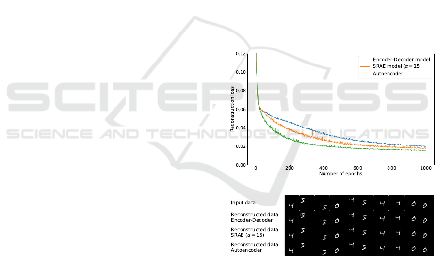
The resulting learning curves with respect to the
reconstruction error are plotted in Figure 1a. The
smallest reconstruction error is achieved by the au-
toencoder with whitened latent factors, followed by
the SRAE model with a weighting factor of α = 15
and the Encoder-Decoder model. From a global per-
spective, all three models show qualitatively similar
monotonically falling learning curves with clear con-
vergence behavior. The autoencoder with whitened
latent variables converges fastest, while the Encoder-
Decoder model converges most slowly.
These results show that the quality of the recon-
structions is inhibited and reduced by restricting the
latent factors to slowly varying features, however,
these effects can be considered to be within an accept-
able range, as the reconstruction errors and the direct
comparison of reconstruction examples of the models
given in Figure 1b demonstrate.
(a)
(b)
Figure 1: Progression of the reconstruction error (a) and re-
constructions (b) of the Encoder-Decoder model, the SRAE
model with weighting factor α = 15 and an autoencoder
with whitened latent variables on a dataset with variation
in position and identity.
The results of this experiment further indicate that
the SRAE model with different weighting factors α
enables an interpolation between an autoencoder and
the Encoder-Decoder model. In an additional anal-
ysis, provided in Appendix B, we trained and com-
pared several SRAE models with different weighting
Exploring Slow Feature Analysis for Extracting Generative Latent Factors
123

factors α and could show that this is indeed the case.
As the weighting of the SFA loss within the composite
loss of the SRAE model increases, the SFA loss de-
creases while the reconstruction loss increases. Based
on this analysis, we further deduce that a weighting
factor of α = 15 offers a good compromise between a
small reconstruction error and the extraction of slowly
varying latent factors.
3.4 Latent Factors and Reconstructions
In this section, we analyze the extracted latent factors
and the structure of the latent space, in particular, with
regard to its continuity, completeness and complex-
ity introduced by dependencies between the individ-
ual latent factors. By the term continuity, we denote
the property that two close points in the latent space
result in two similar reconstructions, while the term
completeness refers to the existence of a meaningful
reconstruction for each point in the latent space.
3.4.1 Explorations on Static Sequences
At first, embeddings and reconstructions of static
sequences are considered. As an initial investiga-
tion of the continuity and completeness of the la-
tent space, we perform a latent space exploration on
four different models. We use the Encoder-Decoder
model and the SRAE model with weighting factor
α = 15. In addition, two autoencoders, one with
and one without whitening of the latent variables,
are trained. These autoencoders therefore correspond
to the SRAE model with or respectively without the
PowerWhitening layer and a weighting factor of α =
0. In all models the latent space has two dimensions.
The dataset for this experiment includes only a
variation in identity. To generate the dataset, we use
five variations of each of the ascending identities from
0 to 9 in succession. The similarity matrix encodes
successive images as similar and connects the identi-
ties 0 and 9. The identity is therefore in this case a
cyclic variable, which can be encoded by two latent
factors. SFA is well-known to extract these factors
when they are clearly reflected in sample similarity.
The latent spaces of the trained models are tra-
versed in 200 equally large steps in both dimen-
sions. For each latent sample, we compare the re-
construction with the input images by calculating the
cross-entropy and assign the most appropriate iden-
tity. The color-coding of the samples represents this
assignment, while the saturation further indicates how
closely the reconstruction matches the assigned input
image. A high saturation indicates a high degree of
correspondence. Figure 2 shows the resulting feature
maps of the four different models.
By comparing the visualizations of the latent
space of the autoencoders (Figure 2a and 2b), it is ev-
ident that the whitening of the latent factors by means
of the PowerWhitening layer leads to a significantly
more compact structure of the latent space. This di-
rectly transfers to a higher degree of completeness
and is also reflected in the reconstruction error on the
training data. Besides the fact that the reconstruction
errors of the autoencoders are overall slightly lower
than those of the models with inclusion of the SFA
objective, it is interesting that the autoencoder includ-
ing the PowerWhitening layer achieves a lower recon-
struction error (0.0127) than the autoencoder without
whitening of the latent factors (0.0156).
Considering the continuity, the local changes of
saturation within and between clusters of different
identities indicate that the identities merge smoothly
and that also continuous transitions between the indi-
vidual variations of an identity exit.
The SFA objective further clearly structures the la-
tent space and arranges the embeddings of the ascend-
ing identities in clockwise order in circular sectors
as the visualizations of the latent space of the SRAE
model (Figure 2c) and Encoder-Decoder model (Fig-
ure 2d) show.
We therefore conclude that the SFA objective
and the associated constraints, implemented in the
SRAE and Encoder-Decoder model, enable a well-
structured, continuous and complete latent space in
the case of data with variation in identity. Experi-
ments on equivalent datasets with variation in rotation
or scaling show qualitatively similar results and sup-
port these statements.
In a further experiment, we analyze more com-
plex datasets with two varying attributes and fo-
cus on the disentanglement of the latent factors as
well as the resulting complexity of the latent space.
We generate two datasets with variation in rotation
(cyclic) in steps of ten degrees and additionally six
different scales (acyclic) or ten different identities
(acyclic). The similarity matrices to these datasets de-
fine a neighborhood-based relationship. Images with
successive rotation, scaling or identity attributes are
therefore encoded as similar. On these two datasets,
we train the SRAE model with three latent factors.
Figure 3 shows the embeddings of the two con-
sidered datasets. In both embeddings the rotation is
encoded in the first two dimensions, while the scaling
or respectively the identity is embedded in the third
dimension.
For the data with variation in rotation and scaling,
the latent factors are strongly disentangled and only
a slight proportional dependence between the radii of
the cyclic embedding of the rotation and the scaling
ICPRAM 2021 - 10th International Conference on Pattern Recognition Applications and Methods
124
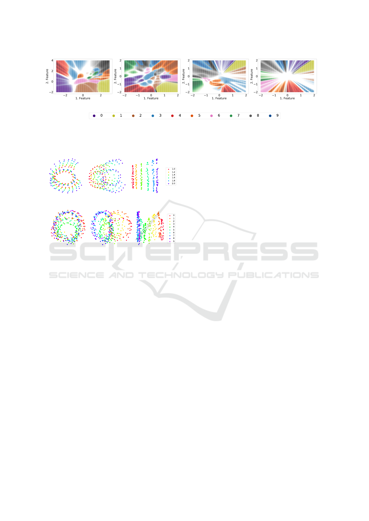
(a) (b) (c) (d)
Figure 2: Visualization of the latent space of the autoencoder (a), autoencoder with PowerWhitening layer (b), SRAE model
(α = 15) (c) and Encoder-Decoder model (d) trained on a dataset including ten different identities in five variations each.
The color-coding of the individual samples represents the corresponding identity, while the saturation indicates the degree of
correspondence.
(a)
(b)
Figure 3: Three views of the embedding of the datasets with
variation in rotation and scaling (a) and variation in rotation
and identity (b).
is visible. The spiral shape of the generally circu-
lar structure of the embedding can be attributed to
strong structural similarities among certain rotations
of the used identity 4. We further note that the embed-
ding computed in this example matches the embed-
dings and results of the coding of the NORB dataset
with similar data-generating factors as computed and
presented in (Sch
¨
uler et al., 2019) qualitatively well.
Based on the unique embedding of the training data,
the decoder is also able to reconstruct the data accu-
rately.
In the embedding of the data with variation in ro-
tation and identity, the embeddings of some identities
overlap and are thus not uniquely encoded with re-
spect to the third dimension. Furthermore, the radii
of the circular embedding of the rotation seem to de-
pend more strongly on the respective identity. This
ambiguity of the embedding is also reflected in poor
reconstructions of the input data.
(Turner and Sahani, 2007) identify a possible
weakness of the standard SFA formulation in that
it confounds categorical and continuous latent fac-
tors during extraction, which might be a reason for
the aforementioned ambiguity. We try to address
this possible weakness by further development of the
Encoder-Decoder model in Section 3.4.3.
3.4.2 Explorations on Moving Sequences
Analogous to the analyses on the static sequences,
we also investigate the embeddings of the moving se-
quences. In addition to the variation of the position,
the rotation or alternatively the identity is varied in
this case. For this purpose the position is chosen from
a grid structure consisting of 18×18 points, the orien-
tation (cyclic) is changed in steps of 20 degrees and
the identity (acyclic) is varied between 0 and 9. For
both datasets, the neighborhood-based method is used
to determine the similarity matrix. We have trained
both the SRAE model as well as the Encoder-Decoder
model on these two datasets. Since the results are al-
most identical, we discuss here only the embeddings
and reconstructions of the SRAE model.
Figure 4 shows the embeddings of the two con-
sidered datasets in the three-dimensional latent space.
The global structure of these embeddings has the form
of a rectangular hyperbolic paraboloid. When project-
ing these embeddings onto the plane spanned by the
first and third dimension, a grid-shaped coding of the
18×18 positions can be identified.
In the case of the dataset with variation in position
and rotation, each node of the grid consists of a lo-
cal structure, which encodes the rotation, as apparent
from the color-coding. The individual embeddings
within the local structure are arranged in a continuous
manner with respect to the corresponding rotation and
reflect the global structure by forming a hyperbolic
paraboloid. These structures on both global and local
scales blur towards the edges of the latent space.
In contrast, no clear local structure can be identi-
fied in the embedding of the dataset with variation in
position and identity. The individual regions appear
much more disorganized and we could not identify a
principal structure of the embedding of the identities.
Exploring Slow Feature Analysis for Extracting Generative Latent Factors
125
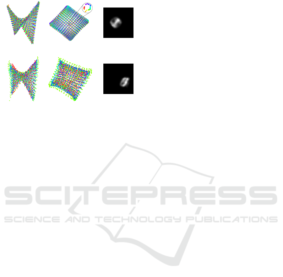
(a)
(b)
Figure 4: Front and top view of the embedding as well as
a single exemplary reconstruction of the datasets with vari-
ation in position and rotation (a) and variation in position
and identity (b).
Overall, the embeddings of the considered mov-
ing sequences form complex structures with strong
dependencies between the latent factors. These hi-
erarchical structures may be due to strongly differing
levels of slowness of the data-generating factors. It
is conceivable that the variation of the position com-
pared to the variation of the rotation or identity results
in features that are significantly slower and there-
fore easier to extract. Additionally, the combination
of continuous and categorical attributes in the case
of the dataset with variation in position and identity
could also impede the formation of a local structure.
Through further experiments with higher dimensional
latent spaces, we could exclude the restriction to three
dimensions as a reason for such embeddings. The ex-
emplary reconstructions demonstrate that the position
is precisely reconstructed, while the rotation or iden-
tity can hardly be recovered at all. The decoder is
therefore not able to learn any exact mapping of the
hierarchical encoding of the varying attributes to cor-
responding reconstructions.
3.4.3 Separated Extraction of Latent Factors
In this section, we introduce an approach for the sep-
arated extraction of continuous and categorical data-
generating attributes. Neither the SFA optimization
problem nor the associated algorithms provide or con-
sider such a separation. The aim of this differentiation
is to achieve a better structuring and stronger disen-
tanglement of the latent factors as well as a better re-
constructability.
This approach is motivated by the observations of
the previous experiments on the static and moving se-
quences and is biologically plausible. Furthermore,
a first theoretical approach along these lines has al-
ready been presented in (Turner and Sahani, 2007),
which, in contrast to our approach, augments the set
of continuous latent variables within a probabilistic
SFA model by a set of binary variables and does not
implement an explicitly separated extraction.
We implement this approach by extending the
Encoder-Decoder model and analyze it in the context
of moving sequences with variation in 36×36 posi-
tions and the identities from 0 to 9. In more general
terms, the data is therefore composed of the categor-
ical attribute of the object identity, which can also be
described as the “What” information, and the contin-
uous attribute of the object position, also referred to
as the “Where” information.
The main idea is based on the separation of the ex-
traction of the features by using two encoders. One of
them is trained to extract continuous features whereas
the other one is trained to extract categorical features.
Applied to the dataset used here, this results in a
What-Encoder, which extracts the identity in a single
feature, and a Where-Encoder, which is responsible
for encoding the position within two features. The ex-
tracted latent factors are then combined to define the
latent space with corresponding continuous and cate-
gorical dimensions. Finally, the decoder reconstructs
the data based on the samples of this combined latent
space.
For the successful implementation of this model,
the training of the encoders is of particular relevance.
For both encoders, we use the identical image data
but specific similarity matrices. To train the What-
Encoder, all images with the same identity indepen-
dent of their position are encoded as similar. The sim-
ilarity matrix for the Where-Encoder encodes those
images as similar which differ in their positioning
only by a maximum of two pixels independent of the
respective identity. The decoder is finally trained on
the combined latent space and the corresponding in-
put images.
Considering the embedding of the dataset plotted
in Figure 5a, a simple and unique encoding of the data
can be observed. The first two latent factors encode
the position, whereas the identities are encoded by
discrete values along the third dimension, as appar-
ent from the color-coding. The latent factors are thus
strongly disentangled and only a slight proportional
dependence between the scale of the position coding
and the third dimension is visible. Such dependencies
can be easily addressed by constructing an adequate
sampling model, as illustrated in Section 3.5.1. Fig-
ure 5b further demonstrates that the samples of the
latent space can be meaningfully reconstructed by the
decoder.
ICPRAM 2021 - 10th International Conference on Pattern Recognition Applications and Methods
126
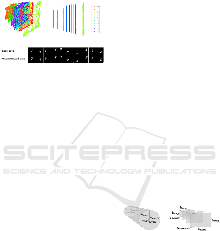
(a)
(b)
Figure 5: Two different views of the combined embedding
(a) of the dataset with variation in position and identity com-
puted by the What- and Where-Encoder as well as exem-
plary reconstructions (b) computed on the basis of the la-
tent samples by the decoder of the What-Where Encoder-
Decoder model.
We conclude that this approach allows the gen-
eration of a simple and well-structured latent space
whose samples can be reconstructed with high pre-
cision by the decoder. Especially in comparison to
the results obtained in the last Section 3.4.2 using the
SRAE model trained on a slightly simpler but nearly
identical dataset, significant improvements in both en-
coding as well as decoding are achieved by using the
What-Where Encoder-Decoder model.
These results therefore support the hypothesis
that a separated extraction and segregated treatment
of continuous and categorical variables is a reason-
able approach to compute structural simple and dis-
entangled embeddings. In the case of the mov-
ing sequences considered in this experiment, addi-
tionally, the otherwise dominant variation in posi-
tion is extracted separately and thereby avoids inhibi-
tions and deterioration of the extraction of other data-
generating attributes.
This approach is, of course, not limited to the data-
generating attributes considered in this example, but
can also be generalized and applied to or extended
by other varying attribute combinations. We assume
that, in particular, the complexity of the latent space
in terms of dependencies between the latent factors in-
creases only moderately when adding further varying
attributes, due to the disentanglement of these factors
obtained by the separated extractions.
A limitation and prerequisite of this approach re-
sults from the additionally required information about
the relations of the training images to compute the dif-
ferent similarity matrices used to train the individual
encoders. However, it should be noted that even a par-
tially separated extraction according to the available
information might lead to significantly better results
and therefore be useful.
3.5 Prior Distributions and Data
Generation
For one of the main goals of generative models – the
generation of new data – the prior distribution over
the latent factors is a key element, since it determines
in which way samples are drawn from the latent space
and accordingly new data is generated. SFA in gen-
eral and explicitly the models presented in this paper
provide latent factors but no prior distribution over
these factors, as no complete probabilistic model for
(non-linear) SFA is known. In this section, we there-
fore present two approaches to generate new mean-
ingful data on the basis of these extracted latent fac-
tors.
3.5.1 Definition of Prior Distributions over
Latent Factors
Motivated by the results of Section 3.4, we define
parameterized prior distributions, which are subse-
quently fit to the latent factors of a concrete dataset.
These prior distributions are constructed based on
characteristic structures identified in the previous sec-
tions. Specifically, different combinations of cyclic
and acyclic variables result in distinct embeddings.
One example for this is the elliptic conical frustum
as the consequence of variations in rotation and scale.
This is supported by structurally similar embeddings
found in (Sch
¨
uler et al., 2019). For sequences with
variation in position and identity, the What-Where
Encoder-Decoder model provides an embedding that
can be well described by a rectangular frustum with
multiple rectangular layers. Figure 6 visualizes these
structures.
(a) (b)
Figure 6: Parameterized fundamental structures in form of a
hollow conical frustum with elliptical bases (a) and a rectan-
gular frustum consisting of multiple rectangular layers (b)
used to define the prior distributions.
Points in both structures can be parameterized by
a small set of parameters. For static sequences, we
can build a prior distribution by assuming indepen-
dent uniform distributions along the height of the frus-
tum and the angle on the elliptical base. The pa-
rameter set therefore consists of the interval limits
[min
acyclic
, max
acyclic
] of the continuous uniform dis-
tribution along the height and the two pairs of radii
Exploring Slow Feature Analysis for Extracting Generative Latent Factors
127

r
min
and r
max
of the elliptical bases. A sample z =
(z
1
, z
2
, z
3
)
T
in latent space is then given by
z
1
= cos(φ) · r
1
, (5a)
z
2
= sin(φ) · r
2
, (5b)
z
3
∼ U (min
acyclic
, max
acyclic
) (5c)
with φ ∼ U (−π, π) (5d)
and (r
1
, r
2
)
T
= h · (r
max
− r
min
) + r
min
, (5e)
h =
z
3
− min
acyclic
max
acyclic
− min
acyclic
. (5f)
For the data based on the moving sequences,
the prior distribution consists of two continuous
as well as one discrete uniform distribution. The
parameter set is composed by the interval limits
[c
k-means,0
, c
k-means,k−1
] of the discrete uniform distri-
bution over the identities and the altogether four inter-
vals for the two bases b
min
and b
max
. The composition
of a sample z from this defined prior distribution can
be formally described by
z
1
∼ U (s
x, min
, s
x, max
), (6a)
z
2
∼ U (s
y, min
, s
y, max
), (6b)
z
3
∼ D(c
c
c
k-means
) (6c)
with (s
s
s
x
, s
s
s
y
)
T
= h · (b
max
− b
min
) + b
min
, (6d)
h =
z
3
− c
k-means,0
c
k-means,k−1
− c
k-means,0
. (6e)
Note that a rotation to align the distributions with
the coordinate axes has to be learned. Fortunately, this
rotation is a by-product of the Independent Compo-
nent Analysis (ICA) step of the following fitting pro-
cedure. The corresponding inverse is calculated by
default in the used implementation of ICA (Pedregosa
et al., 2011) and is justifiable in terms of computa-
tional costs when the latent space is low-dimensional.
We fit these general parameterized prior distribu-
tions to embedded data by estimating the individual
parameters. The fitting procedure developed and ap-
plied for this purpose consists of four steps:
1. Embedding the data,
2. finding rotation and inverse,
3. identifying cyclic/acyclic and discrete/continuous
dimensions,
4. estimating parameters.
The embedded data is first rotated to align the dis-
tributions with the coordinate axes by ICA. Note that
due to the SFA constraints the embedding does not
need to be whitened beforehand.
To determine continuous and categorical dimen-
sions, we first build a 100-bin histogram for each axis.
Afterwards, the axis is either classified as discrete or
continuous depending on the variance over the fre-
quency per bin. Using this heuristic, we are able to
reliably distinguish between continuous and categor-
ical dimensions by a hard threshold. Cyclicity is de-
termined by thresholding the variance for each axis
over the distances from the respective axis to all data
points, with an acyclic variable being coded along the
axis with the smallest variance. Thus, each axis is
matched with one marginal distribution.
Subsequently, the parameters of each marginal
can be estimated directly from the rotated embedding.
The interval limits of continuous uniform distribu-
tions are given by the minimum and maximum values
of the respective dimension. For each categorical di-
mension, we perform k-means clustering to identify
the corresponding discrete values over which a uni-
form distribution is defined. We set the mean values
of the distances to the acyclic axis of the points at the
ends of the conical frustum as the radii of the ellipses.
To sample from the thus fitted prior distributions,
samples are drawn from each marginal and then back-
transformed by the inverse of the rotation matrix pre-
viously determined by ICA in order to align them with
the original embedding.
Figure 7 visualizes the latent space with the two
considered embedded datasets (orange) and samples
taken from the defined and fitted prior distributions
(blue). The samples show that the parameters have
been well estimated and the fitted prior distributions
accurately abstract the embedding of the datasets. To
generate new image data, we use the decoder to de-
code the drawn latent samples. The resulting images
shown in Figure 7 demonstrate that the samples from
the prior distribution represent all variations and can
be decoded meaningfully and accurately by the de-
coder.
In conclusion, we state that this procedure repre-
sents a practicable approach for the posterior defini-
tion and estimation of a prior distribution over latent
factors in the context of the data considered in this
work. By sampling from the defined prior distribu-
tion and decoding the obtained latent data point, the
generation of a new image accurately matching the
original input images is enabled.
This method is of course not limited to the data
considered here, but can be applied to any data with
corresponding continuous, categorical and cyclic or
acyclic underlying variables and latent factors. As-
suming a sufficiently powerful extraction, the charac-
teristic distributions defined here should be applica-
ble.
ICPRAM 2021 - 10th International Conference on Pattern Recognition Applications and Methods
128
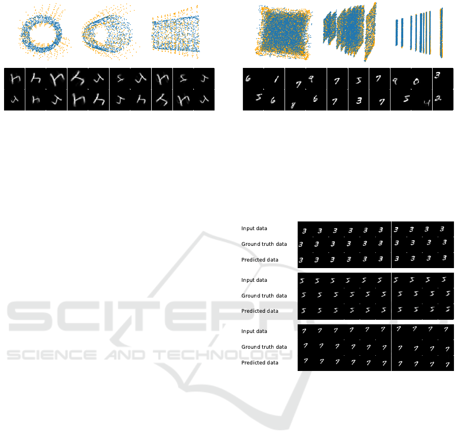
(a) (b)
Figure 7: Three views of the embedding (orange) and latent samples drawn from the fitted prior distribution (blue) as well as
exemplary generated images based on these latent samples of data with variation in rotation and scaling (a) and variation in
position and identity (b).
3.5.2 Prediction of Latent Samples for Sequence
Generation
In this last section, we present an approach for
generating not only single images but whole image
sequences. We extend the Encoder-Decoder model
by a predictor over the latent factors. The predictor is
embedded between the encoder and the decoder and
receives ten successive features as an input sequence.
This input is passed through two layers consisting
of 64 and 32 Long Short Term Memory (LSTM)
units. After applying the ReLU activation function,
the output is reshaped into a sequence of ten features
which are finally fed into the decoder to generate an
image sequence.
To train the predictor, we optimize the parameters
with respect to the mean absolute error between the
predicted sequences and the target sequences using
the stochastic gradient-based RMSprop optimization
method (Tieleman and Hinton, 2012).
We have analyzed the resulting Encoder-
Predictor-Decoder model on different datasets in the
context of both static and moving sequences. In the
following, the results obtained by training on data
with variation in position and within a set of ten
identities are presented. For this purpose, we embed
the predictor into the What-Where Encoder-Decoder
model. The sequences of the dataset consist of 20
images each, where the first half is used as the input
sequence and the second half as the target sequence.
Considering the validation and test error of the
predictor, it can be summarized that based on the
input sequences, the predictor accurately predicts the
ten following features. The output images computed
by the decoder reconstruct the position and identity
in the individual images qualitatively well and the
attributes change smoothly and conclusively in
the course of the sequence. The predicted image
sequence thus corresponds precisely to the respective
ground truth and continue the input sequence in a
reasonable and conclusive way as shown in Figure 8.
Qualitatively similar results could also be achieved
on datasets with other varying attributes.
Figure 8: Image sequences generated by the decoder of the
What-Where Encoder-Decoder model based on predicted
samples for data with variation in position and identity.
We summarize that by extending the Encoder-
Decoder model by a predictor for predicting latent
features, precise and meaningful image sequences can
be generated. These results therefore support the hy-
pothesis that the features extracted by SFA are suit-
able as a basis not only for the generation of single
images as shown in Section 3.5.1, but also for the gen-
eration of sequences of images.
Note that the prediction of image sequences based
on predicted latent feature values offers two elemen-
tary advantages compared to a prediction directly on
the input data. First, the predictor only has to learn
and predict the abstract underlying dynamics in the
low-dimensional latent space. Second, the quality of
the generated images always remains the same and no
distortions or blurring can occur as in some other ap-
proaches due to the collapse of complex LSTMs.
Exploring Slow Feature Analysis for Extracting Generative Latent Factors
129

4 DISCUSSION
In this paper, we explored SFA for the extraction
of generative latent factors. We developed different
models and evaluated them on a variety of datasets
with different data-generating attributes. In this eval-
uation, we found that the extraction principle of slow-
ness is in general not contrary to reconstructability
from low-dimensional representations, while provid-
ing the corresponding space with additional proper-
ties beneficial for generative tasks as has been demon-
strated in Section 3.4. However, while slow features
live in a structured, continuous and complete space,
the specific nature of the extracted features is gov-
erned by the types of latent variables used in data gen-
eration and can negatively impact the overall quality
of the reconstruction in specific cases.
One of these cases is identified as the mixing of
continuous with categorical latent variables and is
subsequently addressed in Section 3.4.3 by develop-
ment of the What-Where Encode-Decoder model us-
ing two qualitatively different extraction paths.
Finally, to complete a possible generative model
based on SFA, a prior distribution had to be con-
structed. As construction of suitable prior distribu-
tions is in general a hard problem, the chosen ap-
proach leveraged known structural properties of SFA-
extracted features and was successfully applied for
the case of single samples of a synthetic dataset
when using a low-dimensional feature space in Sec-
tion 3.5.1. A possible ansatz to also generate se-
quences was discussed in Section 3.5.2.
Future Directions. We see potential in continued
investigation of SFA representations as foundation for
generative models, as it also has been shown to ex-
tract useful representations even in the case of high-
dimensional data. One limitation here might lie in the
use of very low-dimensional latent spaces: While ef-
fective prior distributions can be constructed, not all
interesting latent factors might be captured. There-
fore, the authors regard the possible generalization of
the identified construction principles to higher dimen-
sions as the most promising research direction at this
point.
REFERENCES
B
¨
ohmer, W., Gr
¨
unew
¨
alder, S., Nickisch, H., and Ober-
mayer, K. (2011). Regularized sparse kernel slow
feature analysis. In Gunopulos, D., Hofmann, T.,
Malerba, D., and Vazirgiannis, M., editors, Machine
Learning and Knowledge Discovery in Databases,
pages 235–248, Berlin, Heidelberg. Springer Berlin
Heidelberg.
Denton, E. and Fergus, R. (2018). Stochastic video gener-
ation with a learned prior. In Dy, J. and Krause, A.,
editors, Proceedings of the 35th International Confer-
ence on Machine Learning, volume 80 of Proceedings
of Machine Learning Research, pages 1174–1183,
Stockholmsm
¨
assan, Stockholm Sweden. PMLR.
Dozat, T. (2015). Incorporating nesterov momentum into
adam. http://cs229.stanford.edu/proj2015/054
report.
pdf.
Escalante-B, A. N. and Wiskott, L. (2020). Improved graph-
based sfa: Information preservation complements the
slowness principle. Machine Learning, 109(5):999–
1037.
Franzius, M., Sprekeler, H., and Wiskott, L. (2007). Slow-
ness and sparseness lead to place, head-direction,
and spatial-view cells. PLoS Computational Biology,
3(8):1–18.
Franzius, M., Wilbert, N., and Wiskott, L. (2011). Invariant
object recognition and pose estimation with slow fea-
ture analysis. Neural Computation, 23(9):2289–2323.
Goodfellow, I., Bengio, Y., and Courville, A. (2016). Deep
Learning. MIT Press. http://www.deeplearningbook.
org.
Goodfellow, I., Pouget-Abadie, J., Mirza, M., Xu, B.,
Warde-Farley, D., Ozair, S., Courville, A., and Ben-
gio, Y. (2014). Generative adversarial nets. In Ghahra-
mani, Z., Welling, M., Cortes, C., Lawrence, N. D.,
and Weinberger, K. Q., editors, Advances in Neu-
ral Information Processing Systems 27, pages 2672–
2680. Curran Associates, Inc.
Hafner, D., Lillicrap, T., Ba, J., and Norouzi, M. (2020).
Dream to control: Learning behaviors by latent imag-
ination. In International Conference on Learning Rep-
resentations.
Karras, T., Aila, T., Laine, S., and Lehtinen, J. (2018). Pro-
gressive growing of GANs for improved quality, sta-
bility, and variation. In International Conference on
Learning Representations.
Kingma, D. P. and Ba, J. (2014). Adam: A
method for stochastic optimization. arXiv preprint
arXiv:1412.6980.
Kingma, D. P., Salimans, T., Jozefowicz, R., Chen, X.,
Sutskever, I., and Welling, M. (2016). Improved vari-
ational inference with inverse autoregressive flow. In
Advances in neural information processing systems,
pages 4743–4751.
Kingma, D. P. and Welling, M. (2013). Auto-encoding vari-
ational bayes. arXiv preprint arXiv:1312.6114.
Kingma, D. P. and Welling, M. (2019). An introduction to
variational autoencoders. Foundations and Trends
R
in Machine Learning, 12(4):307–392.
LeCun, Y., Cortes, C., and Burges, C. (2010). Mnist hand-
written digit database. http://yann.lecun.com/exdb/
mnist.
Mehri, S., Kumar, K., Gulrajani, I., Kumar, R., Jain, S.,
Sotelo, J., Courville, A., and Bengio, Y. (2016). Sam-
plernn: An unconditional end-to-end neural audio
generation model. arXiv preprint arXiv:1612.07837.
ICPRAM 2021 - 10th International Conference on Pattern Recognition Applications and Methods
130
Pedregosa, F., Varoquaux, G., Gramfort, A., Michel, V.,
Thirion, B., Grisel, O., Blondel, M., Prettenhofer,
P., Weiss, R., Dubourg, V., Vanderplas, J., Passos,
A., Cournapeau, D., Brucher, M., Perrot, M., and
Duchesnay, E. (2011). Scikit-learn: Machine learning
in Python. Journal of Machine Learning Research,
12:2825–2830.
Sch
¨
uler, M., Hlynsson, H. D., and Wiskott, L. (2019).
Gradient-based training of slow feature analysis by
differentiable approximate whitening. In Lee, W. S.
and Suzuki, T., editors, Proceedings of The Eleventh
Asian Conference on Machine Learning, volume 101
of Proceedings of Machine Learning Research, pages
316–331, Nagoya, Japan. PMLR.
Srivastava, N., Mansimov, E., and Salakhudinov, R. (2015).
Unsupervised learning of video representations using
lstms. In International conference on machine learn-
ing, pages 843–852.
Sutton, R. S. and Barto, A. G. (2018). Reinforcement learn-
ing: An introduction. MIT press.
Tieleman, T. (2013). The affnist dataset. www.cs.toronto.
edu/
∼
tijmen/affNIST/.org.
Tieleman, T. and Hinton, G. (2012). Lecture 6.5-rmsprop:
Divide the gradient by a running average of its recent
magnitude. COURSERA: Neural networks for ma-
chine learning, 4(2):26–31.
Tulyakov, S., Liu, M.-Y., Yang, X., and Kautz, J. (2018).
Mocogan: Decomposing motion and content for video
generation. In Proceedings of the IEEE conference on
computer vision and pattern recognition, pages 1526–
1535.
Turner, R. and Sahani, M. (2007). A maximum-likelihood
interpretation for slow feature analysis. Neural Com-
putation, 19(4):1022–1038.
Van den Oord, A., Dieleman, S., Zen, H., Simonyan,
K., Vinyals, O., Graves, A., Kalchbrenner, N., Se-
nior, A., and Kavukcuoglu, K. (2016a). Wavenet:
A generative model for raw audio. arXiv preprint
arXiv:1609.03499.
Van den Oord, A., Kalchbrenner, N., Espeholt, L., Vinyals,
O., Graves, A., et al. (2016b). Conditional image gen-
eration with pixelcnn decoders. In Advances in neural
information processing systems, pages 4790–4798.
Wiskott, L. and Sejnowski, T. (2002). Slow feature anal-
ysis: Unsupervised learning of invariances. Neural
Computation, 14(4):715–770.
Yarats, D., Zhang, A., Kostrikov, I., Amos, B., Pineau,
J., and Fergus, R. (2019). Improving sample effi-
ciency in model-free reinforcement learning from im-
ages. arXiv preprint arXiv:1910.01741.
APPENDIX
A Architectures and Code
Further details on the models, datasets and experi-
ments can be found at https://github.com/m-menne/
slow-generative-features.
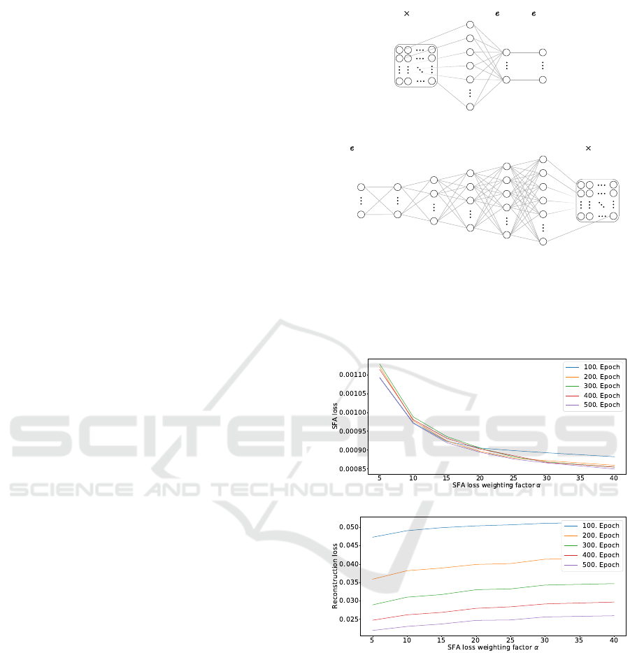
4096units512units
Hiddenlayers
256units128units64units
Outputlayer
64 64units
Inputlayer
units
Hiddenlayers
4096units units
Inputlayer
64 64units
Outputlayer
units
(a)
4096units512units
Hiddenlayers
256units128units64units
Outputlayer
64 64units
Inputlayer
units
(b)
Figure 9: Architecture of the encoder (a) and decoder (b)
network used in the different models.
B Influence of the Weighting Factor α
(a)
(b)
Figure 10: SFA loss (a) and reconstruction loss (b) in re-
lation to the SFA weighting factor α after training for 100,
200, 300, 400 and 500 epochs.
Exploring Slow Feature Analysis for Extracting Generative Latent Factors
131
