
Convolution-based Soma Counting Algorithm for Confocal Microscopy
Image Stacks
Shih-Ting Huang, Yue Jiang and Hao-Chiang Shao
a
Department of Statistics and Information Science, Fu Jen Catholic University, Taiwan, Republic of China
Keywords:
Neuroblast, Soma Detection, Drosophila Brain, Confocal Microscopy.
Abstract:
To facilitate brain research, scientists need to identify factors that can promote or suppress neural cell differ-
entiation mechanisms. Accordingly, the way to recognize, segment, and count developing neural cells within
a microscope image stack becomes a fundamental yet considerable issue. However, it is currently not feasible
to develop a DCNN (deep convolutional neural network) based segmentation algorithm for confocal fluores-
cence image stacks because of the lack of manual-annotated segmentation ground truth. Also, such tasks
traditionally require meticulous manual preprocessing steps, and such manual steps make the results unstable
even with software support like ImageJ. To solve this problem, we propose in this paper a convolution-based
algorithm for cell recognizing and counting. The proposed method is computationally efficient and nearly
parameter-free. For a 1024 × 1024 × 70 two-channel image volume containing about 100 developing neuron
cells, our method can finish the recognition and counting tasks within 250 seconds with a standard deviation
smaller than 4 comparing with manual cell-counting results.
1 INTRODUCTION
Biological labs need to identify factors, including
gene fragments, that can promote or suppress neural
cell differentiation mechanisms to facilitate brain re-
search. To understand the impact of the transplanted
gene fragment on neurodevelopment, the difference
of the number of neural cells between the wild type,
i.e., the phenotype of the typical form of a species
as it occurs in nature, and a mutant, i.e., the indi-
vidual with transplanted RNA interference fragments,
should be clarified. Hence, the way to recognize,
segment, and count developing neural cells within
a microscope image volume becomes a fundamental
yet considerable issue. However, it is currently not
feasible to segment these kinds of confocal fluores-
cence image volumes by using convolutional neural
networks (CNN), such as U-Net (Ronneberger et al.,
2015) or 3D U-Net (C¸ ic¸ek et al., 2016), because of
i) the lack of labeled segmentation ground truth and
ii) the oversized confocal image volumes. Also, such
tasks traditionally require meticulous manual steps,
so the results cannot be stable even with software sup-
port like ImageJ (Ima, 2020). To settle down this
problem, we propose in this paper an algorithm for
a
https://orcid.org/0000-0002-3749-234X
cell recognizing and counting based on convolutional
operators and conventional image processing skills.
The proposed method is computationally efficient,
nearly parameter-free, and aims to extract trustworthy
segmentation ground truth for developing advanced
CNN-based algorithms. For a 1024 × 1024 × 70 fo-
cal stack, focused on the calyx of the mushroom body
in the Drosophila brain, containing about 100 devel-
oping neuron cells, our method can finish the recog-
nition and counting tasks within 240 seconds with a
standard deviation smaller than 4 comparing with the
manual cell-counting results. To process this kind of
confocal image volume, the current standard is still
a computer-aided manual procedure, for instance, us-
ing common software including ImageJ (Ima, 2020)
and Imaris (ima, 2020). However, these programs
require manual input, and therefore they cannot pro-
vide reliable results if the user does not have sufficient
anatomical knowledge of the fly brain and neurons.
In addition, because for confocal microscopy imag-
ing the sampling interval on the z-axis is usually three
times the sampling interval on the x- and the y- axes,
it is difficult and time-consuming to clarify the rela-
tionship between soma candidates on adjacent slices.
Therefore, we proposed this method to segment and
count neuroblast cells.
Huang, S., Jiang, Y. and Shao, H.
Convolution-based Soma Counting Algorithm for Confocal Microscopy Image Stacks.
DOI: 10.5220/0010388403510356
In Proceedings of the 14th International Joint Conference on Biomedical Engineering Systems and Technologies (BIOSTEC 2021) - Volume 4: BIOSIGNALS, pages 351-356
ISBN: 978-989-758-490-9
Copyright
c
2021 by SCITEPRESS – Science and Technology Publications, Lda. All rights reserved
351
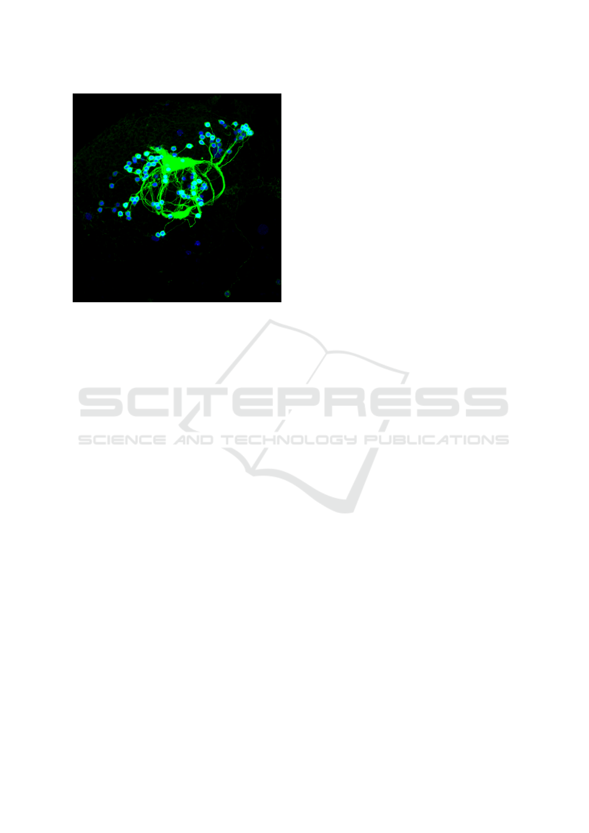
Figure 1: Maximum intensity projection (MIP) of an exam-
ple confocal fluorescence image volume. Red balls are neu-
ron cell bodies (soma), green channel records neural fibres
and cell membranes, and dark red areas are background tis-
sues of fly brain. Note that in order to avoid confusion in red
and green channels, we illustrate all MIP images by swap-
ping blue and red channels later in this paper. Note that in
this figure we render the RED channel in blue so that even
color-blind readers can distinguish soma from neural fibers
and membranes.
2 RELATED WORK
To process 2D+Z confocal fluorescence image vol-
umes, several methods were proposed. However,
most of them focus on image atlasing and surface reg-
istration (Chen et al., 2012; Shao et al., 2013; Shao
et al., 2014), a few of them describe segmentation
strategies on neuron fibers and neuropils (Shao et al.,
; Shao et al., 2019), but none of them depicts soma
(cell body) identification methods. Although in (Shao
et al., ) Shao et al. trace neural fibers within a brain-
bow/flybow (Livet et al., 2007; Hadjieconomou et al.,
2011) image volume by identifying soma candidates
first (Shao et al., ), their method lacks a mechanism
to rule out false somas so that it is hard for their
method to separate independent neurons. In addition,
Shao and his co-authors also stated in (Shao et al.,
2011) and (Shao et al., ) that the effectiveness of im-
age processing routines designed for confocal fluores-
cence images may be degraded due to fluorescence
halation. The pin-hole of the confocal microscope
still cannot filter out fluorescence emitted from out-
of-focus planes. Hence, some anti-halation methods
are still necessary for confocal imagery. To remove
halation, Shao et al. adopted morphological top-hat
transfrom in (Shao et al., ). However, this strategy re-
quires a pre-defined marker and a suitable structural
element, so it cannot be robust. Therefore, we fi-
nally decided to utilize the common most deconvo-
lution method, i.e., Lucy-Richardson deconvolution
(Fish et al., 1995), to remove all possible fluerescence
halation due to the imaging point spread function. In
next section, we will describe our method in detail.
3 METHOD
3.1 Overview
A common strategy to detect neuron cell bodies is to
use morphological operations, i.e., erosion and dila-
tion with handcrafted structural elements, as reported
in (Shao et al., ). However, such a strategy is not ro-
bust against noises and therefore needs several post-
processing steps to rule out unqualified candidates of
neuron cell bodies.
The proposed method was designed for two pur-
poses. First, this method was developed to provide
a cell-body identification result that is more stable
than those obtained by manual procedures. Second,
this method was developed to mass-produce cell body
segmentation results for a further study like training
and specializing in a U-net for this application. There-
fore, the proposed method was designed and imple-
mented by using primarily convolutional operations.
3.2 Soma Identifier
To systematically extract neuron cell bodies (soma),
we first derive several W × H × Z feature maps by
convoluting source image volume with several 2D+Z
Gaussian kernels of different σ
i
and window size w
i
.
Practically, each Gaussian kernel is a 3D array with
its entries specified by following equations.
F
i
= I ∗ G
i
(σ
i
,w
i
), (1)
where ∗ denotes 3D convolution, and G
i
is a w
i
× w
i
convolution kernel with entries defined by
G
i
= αe
−X
T
X/σ
2
i
with X
T
= (x, y,3z). (2)
Here, I is the source image volume, F
i
is the fea-
ture map corresponding to the i
th
Gaussian convolu-
tion kernel G(σ
i
,w
i
), and α denotes a constant gain
factor used to normalize G
i
. Note that the factor 3 in
Eq. (2) reflects the sampling interval in the z axis, as
we will describe in Section 4.1.
The aforementioned convolution step can be re-
garded as a template matching process. Consequently,
BIOSIGNALS 2021 - 14th International Conference on Bio-inspired Systems and Signal Processing
352
we can find candidates of neuron cell bodies by iden-
tifying local maximums on all feature map F
i
. By let-
ting δ
i
( j) denote the list recording the j
th
local maxi-
mum of feature map F
i
, this second step aims to find
the intersection set of local maximums of all feature
maps. We use ∆
main
to denote the resulting intersec-
tion set, that is,
∆
main
= ∩
i
δ
i
. (3)
3.3 Halation Suppression
However, neurons cell bodies may be locally-
concentrated near specific neuropils; in this situation,
for example, two close neuron cell bodies would be
entangled on microscopy images and thus usually re-
sult in one ridge, rather than two local maximums, on
the feature map. To overcome this difficulty, we apply
Richardson–Lucy deconvolution (Richardson, 1972)
method to remove the effect of halation in the fluores-
cence image volume so that neuron cell bodies, which
cluster within a small region, becomes distinguish-
able. Then, we repeat the Soma identifier procedure
described in previous subsection by utilizing smaller
convolution kernels, denoted as G
ps f
(σ
ps f
,w
ps f
), and
then detect the local maximums to find cell bodies
candidates again. We use ∆
aux
to denote Cell bod-
ies detected in this stage. Note that Richardson–Lucy
deconvolution method requires a user-specified blur
kernel, i.e., the point spread function (PSF); in our
implementation, the blur kernel used in this step is
also the convolution kernel G
ps f
(σ
ps f
,w
ps f
).
Because Richardson–Lucy deconvolution may en-
hance/highlight imaging noise, fake cell body candi-
dates would be produced after the second convolu-
tional detection procedure. To settle this issue, we
collect experiment results of more than 80 confocal
image volumes, each acquired with different sam-
ple preparation condition and imaging configurations,
and then induce following judgement rules.
• For any two cell body candidates, if the distance
between them is no larger than 10 voxels, we rule
out the one with lower average brightness.
• If a new cell body candidate (derived in the sec-
ond step) does not locate within the bounding box
of any soma candidate obtained in the first step,
we will disregard it unless its average brightness
reaches level of top 1%.
Finally, because we now have only about 80 image
volumes of different geno-types and different imag-
ing parameter settings, all above rules are developed
empirically. We will show our experiment result in
next section.
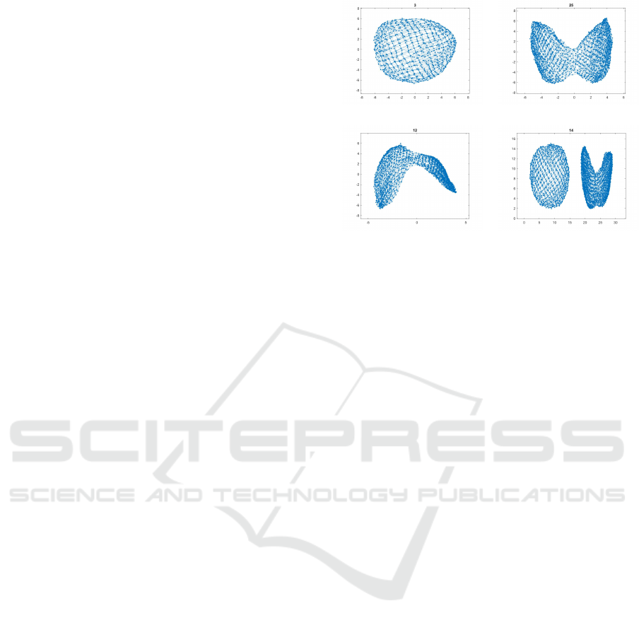
(a) (b)
(c) (d)
Figure 2: Visualized graph of different soma candidates. (a)
a typical graph showing only one soma; (b) a graph show-
ing two concatenated soma; (c) one another example of two
concatenated soma; and, (d) a local graph showing there are
three soma within this area.
3.4 Graph Reconstruction for Manual
Validation
This step is optional in our design; and, it will be ap-
plied if the number of neural cell bodies in the left
brain and that in the right brain are too different. In
this step, we reconstruct and visualize a graph model
for pixels of each extracted soma, and this visualiza-
tion can at least assist users to verify if there are mul-
tiple neural cell bodies within an “extracted soma”.
Demonstrated in Figure 2 are examples of visualized
graphs. Note that these are K-nearest-neighbor (kNN)
graphs derived by taking each pixel’s (x, y, z, inten-
sity) information into account. Through this represen-
tation, we can validate the effective number of somas
within “one soma candidate”, predicted by our algo-
rithm, efficiently.
4 EXPERIMENT RESULT
4.1 Dataset
All source image volumes used in this paper were ac-
quired by an LSM-700 confocal microscope. Each
image volume contains two channels. The red chan-
nel records fluorescence emitted by neuron cell bodies
by using the excitation laser at 555nm, and the green
channel records neuron cell membrane and neuron
fibers by using the excitation laser at 488 nm. The spa-
tial dimension of all image volumes is 1,024× 1,024,
and an image volume may contain about 50 ∼ 100
Convolution-based Soma Counting Algorithm for Confocal Microscopy Image Stacks
353
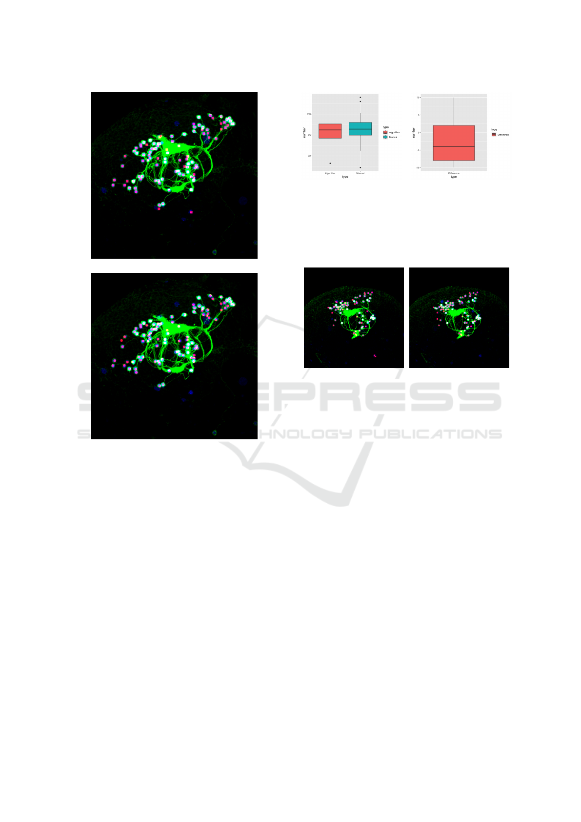
(a)
(b)
Figure 3: Comparison between MIP images of (a) our re-
sult and (b) the manual labeling result of the image volume
shown in Figure 1. The source image volume contains 100
slices.
slices. Note that the actual size of each voxel is about
0.16 × 0.16 × 0.50µm
3
.
4.2 Discussion
Because there is not state-of-the-art or benchmark
method in this field, we compare our segmentation
results with manual counting/labeling results. Figure
3 shows the comparison among the MIP image of one
source volume, the MIP image of our soma identifi-
cation result, and the MIP image of manual labeling
result. Here, red balls are neural cells, green channel
records neural fibres and cell membranes, and dark
red areas are background tissues of fly brain. Note
that we changed the source red-channel that records
neuron cell bodies to the blue-channel so that even
readers with color-vision-deficiency can read our il-
lustrations. Also, summarized in Figure 4 is the sta-
(a) (b)
Figure 4: Statistical comparison. (a) This plot shows that
the average number of extracted soma of the proposed
method is almost the same with that of manual counting
result. (b) This plot shows that the difference between our
segmentation result and manual ground truth mostly rang-
ing from -7.5 to 2.5.
(a) (b)
Figure 5: Comparison between MIP images of the manual
labeling result and our result. This source image volume
contains 82 slices. (a) Result derived by our method. (b)
Manual labelling result.
tistical information of our experiment soma counting
results. Finally, shown in Figures 5 ∼ 9 are results of
other five image volumes.
These experiment results prove that the proposed
method can provide much more stable and reliable
soma counting results than manual process. How-
ever, the proposed method now has two obvious draw-
backs. First, it may misrecognizes other cells as neu-
roblasts once they were labeled by the antibody dur-
ing the stain process. Second, for image volumes with
low brightness, several neuron cell bodies may be dis-
regarded because their voxel intensities are too weak
to hold their contour shape.
5 CONCLUDING REMARKS
In this paper, we proposed a cell-counting proto-
type algorithm for confocal fluorescence image vol-
umes. Compared with time-consuming manual and
software-assisted cell-counting strategies, the pro-
posed method can finish the calculation of a 1024 ×
1024 × 80 image volume within 5 minutes and pro-
vide a better and more stable segmentation and count-
BIOSIGNALS 2021 - 14th International Conference on Bio-inspired Systems and Signal Processing
354
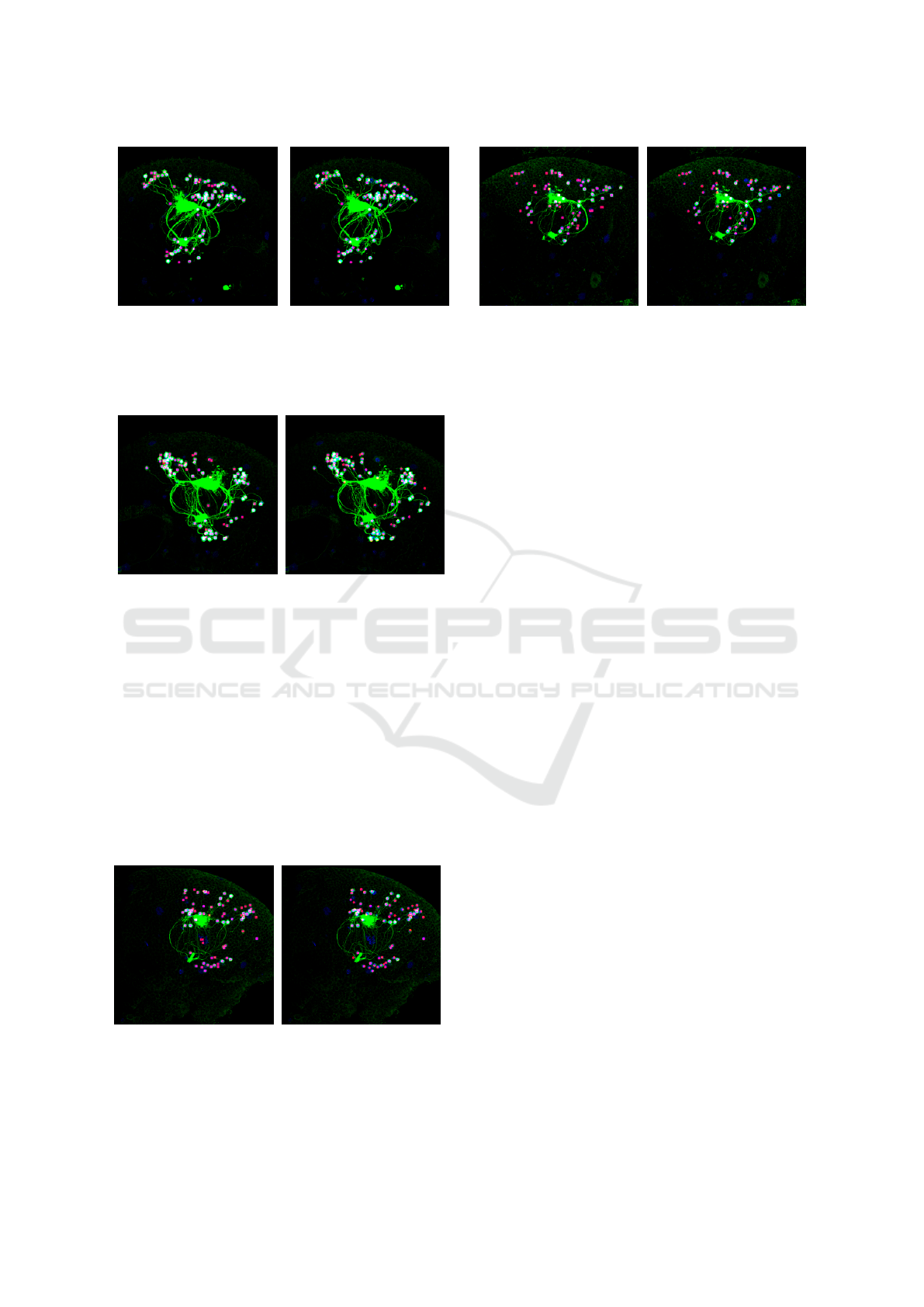
(a) (b)
Figure 6: Comparison between MIP images of the manual
labeling result and our result. This source image volume
contains 83 slices. (a) Result derived by our method. (b)
Manual labelling result.
(a) (b)
Figure 7: Comparison between MIP images of the manual
labeling result and our result. This source image volume
contains 89 slices. (a) Result derived by our method. (b)
Manual labelling result.
ing result. The proposed method has one primary lim-
itation. That is, for flat, disc-shaped neuron cell bod-
ies, especially those with extra-low brightness and ex-
isting on less than three slices, the proposed algorithm
may fail to recognize them.
The proposed algorithm currently may also fail to
recognize flat and disc-shaped cells, especially those
that only exist on less than three slices. We are cur-
rently working on this issue. Also, as for the neurob-
(a) (b)
Figure 8: Comparison between MIP images of the manual
labeling result and our result. This source image volume of
a wide-type contains 76 slices. (a) Result derived by our
method. (b) Manual labelling result.
(a) (b)
Figure 9: Comparison between MIP images of the manual
labeling result and our result. This source image volume
of a wild-type contains 67 slices. (a) Result derived by our
method. (b) Manual labelling result.
last in Drosophila brain, there is still one another sam-
ple preparation method, which is designed for imag-
ing tissue in a very large field of view but labeling
neuron cell membrane only. Hence, one of our future
extensions is to modify our prototype algorithm for
this kind of image.
ACKNOWLEDGEMENT
This work supported by MOST 107-2320-B-030-012-
MY3. The authors want to thank Prof. Hung-Hsiang
Yu from the Institute of Cellular and Organismic Bi-
ology, Academia Sinica, Taiwan for providing the
source confocal microscopy image volumes.
REFERENCES
(2020). Imagej. https://imagej.nih.gov/ij/.
(2020). Imaris. https://imaris.oxinst.com/.
Chen, G.-Y., Wu, C.-C., Shao, H.-C., Chang, H.-M., Chi-
ang, A.-S., and Chen, Y.-C. (2012). Retention of
features on a mapped drosophila brain surface us-
ing a bezier-tube-based surface model averaging tech-
nique. IEEE transactions on biomedical engineering,
59(12):3314–3326.
C¸ ic¸ek,
¨
O., Abdulkadir, A., Lienkamp, S. S., Brox, T.,
and Ronneberger, O. (2016). 3d u-net: learning
dense volumetric segmentation from sparse annota-
tion. In International conf. on medical image comput-
ing and computer-assisted intervention, pages 424–
432. Springer.
Fish, D., Brinicombe, A., Pike, E., and Walker, J. (1995).
Blind deconvolution by means of the richardson–lucy
algorithm. JOSA A, 12(1):58–65.
Hadjieconomou, D., Rotkopf, S., Alexandre, C., Bell,
D. M., Dickson, B. J., and Salecker, I. (2011). Fly-
bow: genetic multicolor cell labeling for neural circuit
analysis in drosophila melanogaster. Nature methods,
8(3):260–266.
Convolution-based Soma Counting Algorithm for Confocal Microscopy Image Stacks
355

Livet, J., Weissman, T. A., Kang, H., Draft, R. W., Lu,
J., Bennis, R. A., Sanes, J. R., and Lichtman, J. W.
(2007). Transgenic strategies for combinatorial ex-
pression of fluorescent proteins in the nervous system.
Nature, 450(7166):56–62.
Richardson, W. H. (1972). Bayesian-based iterative method
of image restoration. JoSA, 62(1):55–59.
Ronneberger, O., Fischer, P., and Brox, T. (2015). U-net:
Convolutional networks for biomedical image seg-
mentation. In International Conference on Medical
image computing and computer-assisted intervention,
pages 234–241. Springer.
Shao, H.-C., Cheng, W.-Y., Chen, Y.-C., and Hwang, W.-L.
Colored multi-neuron image processing for segment-
ing and tracing neural circuits. In 2012 19th IEEE
International Conference on Image Processing, pages
2025–2028. IEEE.
Shao, H.-C., Hwang, W.-L., and Chen, Y.-C. (2011). Opti-
mal multiresolution blending of confocal microscope
images. IEEE transactions on biomedical engineer-
ing, 59(2):531–541.
Shao, H.-C., Wang, Y.-M., and Chen, Y.-C. (2019). A two-
phase segmentation method for drosophila olfactory
glomeruli. In 2019 IEEE International Conf. on Image
Processing (ICIP), pages 265–269. IEEE.
Shao, H.-C., Wu, C.-C., Chen, G.-Y., Chang, H.-M., Chi-
ang, A.-S., and Chen, Y.-C. (2014). Developing a
stereotypical drosophila brain atlas. IEEE Transac-
tions on Biomedical Engineering, 61(12):2848–2858.
Shao, H.-C., Wu, C.-C., Hsu, L.-H., Hwang, W.-L., and
Chen, Y.-C. (2013). 3d thin-plate spline registration
for drosophila brain surface model. In 2013 IEEE In-
ternational Conf. on Image Processing, pages 1438–
1442. IEEE.
BIOSIGNALS 2021 - 14th International Conference on Bio-inspired Systems and Signal Processing
356
