Non-linear Motorcycle Dynamic Model for Stability and Handling

Analysis with Roll Motion and Longitudinal Speed Regulation

Vincenzo Maria Arricale

, Renato Brancati

, Francesco Carputo

, Antonio Maiorano

and Guido Napolitano Dell’Annunziata

Department of Industrial Engineering, University of Naples “Federico II”, Via Claudio 21, Naples, Italy

Keywords: Non-linear Dynamics, Motorcycle Model, Longitudinal Control, Handling Analysis.

Abstract: The use of computer simulations in motorcycle engineering makes it possible both to reduce designing time

and costs and to avoid the risks and dangers associated with experiments and tests. The multi-body model for

computer simulations can be built either by developing a mathematical model of the vehicle or by using

commercial software for vehicle system dynamics. Even though the first method is more difficult and time-

consuming than the second, maximum flexibility in the description of the features of the model can be

obtained only by using an analytical model. Moreover, mathematical modelling has a high computation

efficiency, whereas multi-body software requires a lot of time to carry out simulations. For the reasons above,

the aim of this work was to develop a mathematical model of a motorcycle.

1 INTRODUCTION

The goal of many inventors over the past six centuries

was to discover a device for fast and easy road

transport. The invention of motorcycles began after

the development of bicycles and engines. In fact, the

first motorcycles were merely bicycles with small

engines thrust into the frame. Nowadays, as one of the

world’s most popular means of transport, the

motorcycle is not the early period monster that was

made of metal and solid wood; it is rich in variety,

advanced technology and well-made. Compared with

other methods of transport, it has unparalleled

advantages: it is economical, convenient and fast way

to travel far away (Sharp et al., 2001; Herlihy, 2004)

During nearly 130 years of development,

pioneering builders have exhausted their own

intelligence and have created numerous milestone

achievements, leaving their name in the history

books. From the twenties of the 20th century to the

present, improvements have become the main theme

of the development of motorcycles (Limebeer et al.,

2002). The modeling and control of a motorcycle are

https://orcid.org/0000-0002-1292-1566

https://orcid.org/0000-0003-2718-5706

https://orcid.org/0000-0001-8436-2516

https://orcid.org/0000-0002-9321-626X

https://orcid.org/0000-0002-7293-4975

different from the process for a bicycle for three main

reasons. First of all, the weight of a motorcycle is

much larger than that of a bicycle; the difference is

about ten times (Limebeer et al., 2002; Sharp, 1971).

Secondly, due to the disparate weight, the rider has a

different role to play during the model building

process between a motorcycle and a bicycle. Thirdly,

the speed is also hugely different. In fact, usually, the

speed of a bicycle can be around 20 km/h whereas a

modern motorcycle can achieve a top speed of about

230 km/h. For some sport motorcycles, the speed is

able to reach even 300 km/h. Under this speed, the

modeling process should not only consider the normal

dynamics of the bicycle but should also consider the

aerodynamics force analysis and the relevant thermal

phenomena arising during the vehicle motion

(Farroni et al., 2019). Over the years the theory of

motorcycle dynamics has been perfected gradually,

and some scholars have even done experimental

research based on their own experience (Escalona et

al., 2018; Sharp et al., 1980; Spierings, 1981).

The kinematic study of motorcycles is important,

especially in relation to the effects on their dynamic

behavior. Therefore, in this paper, in addition to the

292

Arricale, V., Brancati, R., Carputo, F., Maiorano, A. and Napolitano Dell’Annunziata, G.

Non-linear Motorcycle Dynamic Model for Stability and Handling Analysis with Roll Motion and Longitudinal Speed Regulation.

DOI: 10.5220/0010386802920300

In Proceedings of the 7th International Conference on Vehicle Technology and Intelligent Transport Systems (VEHITS 2021), pages 292-300

ISBN: 978-989-758-513-5

kinematic study, some simple examples of the

dynamic behavior of motorcycles are reported in

order to show how kinematic peculiarities influence

the directional stability and maneuverability of

motorcycles (Bruni et al., 2020; Cossalter, 2014;

Cossalter et al., 2002). Finally, the aim of this work is

the development of a simple and effective motorcycle

model easily implementable in control logics on

board.

2 KINEMATICS OF

MOTORCYCLES

Motorcycles are composed of a great variety of

mechanical parts, including some complex ones.

From a strictly kinematic point of view, by

considering the suspensions to be rigid, a motorcycle

can be defined as simply a spatial mechanism

composed of four rigid bodies (Genta, 1997;

Gillespie, 1996):

▪ The rear assembly (frame, saddle, tank and mοtοr-

transmission drivetrain group);

▪ The front assembly (fork, steering head and

handlebars);

▪ The front wheel;

▪ The rear wheel.

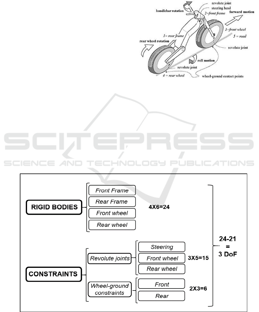
▪ These rigid bodies are connected by three revolute

joints (the steering axis and the two-wheel axles)

and are in contact with the ground at two

wheels/ground contact points as shown in Fig.

1.Each revolute joint inhibits five degrees of

freedom (DoF) in the spatial mechanism, whereas

each wheel-ground contact point leaves three DoF

free (Koenen, 1983; Schwab et al., 2004).

Figure 1: Kinematics representation of a motorcycle

(Cossalter, 2014).

Considering the hypothesis of the pure rolling of tires

on the road to be valid, it is easy to ascertain that each

wheel, with respect to the fixed road, can only rotate

around (Farroni et al., 2019; Kooijman et al., 2011):

▪ The contact point on the wheel plane (forward

motion);

▪ The intersection axis of the motorcycle and road

planes (roll motion);

▪ The axis passing through the contact point and the

centre of the wheel (spin).

Figure 2: Degrees of Freedom of the schematized motorcycle model.

Non-linear Motorcycle Dynamic Model for Stability and Handling Analysis with Roll Motion and Longitudinal Speed Regulation

293

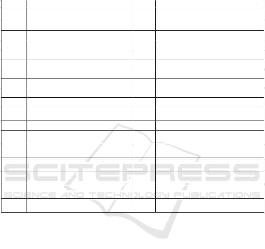
Table 1: List of symbols.

In conclusion, a motorcycle’s number of degrees

of freedom is equal to three, given that the fifteen DoF

inhibited by the three revolute joints and the six

degrees of freedom eliminated by the two wheel-

ground contact points must be subtracted from the

four rigid bodies’ twenty-four DoF, as summarized in

Fig. 2 ( Escalona et al., 2012; Lowell et al., 1982).

These three degrees of freedom may be associated

with three principal motions (Schwab et al., 2004; Yi

et al., 2009):

▪ Forward motion of the motorcycle (represented

by the rear wheel rotation);

▪ Roll motion around the straight line which joins

the tire contact points on the road plane;

▪ Steering rotation.

The rider manages all the three major movements,

according to his personal style and skill: the resulting

movement of the motorcycle and the corresponding

trajectory (e.g. a curve) depend on a combination, in

the time domain, of the three motions related to the

three degrees of freedom. This generates one

manoeuvre, among the thousands possible, which

represents the personal style of the driver. These

considerations have been formulated assuming that

the tires move without slippage. However, in reality,

the tire movement is not just a rolling process. The

generation of longitudinal forces (driving and braking

forces) and lateral forces requires some degree of

slippage in both directions, longitudinally and

laterally, depending on the road conditions. The

number of degrees of freedom is therefore seven

(Dugoff et al., 1969; Pacejka, 2006; Rajput et al.,

2007; Seffen et al., 2001):

▪ Forward motion of the motorcycle;

▪ Rolling motion;

▪ Handlebar rotation;

▪ Longitudinal slippage of the front wheel

(braking);

▪ Longitudinal slippage of the rear wheel (thrust

or braking);

Symbol

Description

Symbol

Description

Rotation matrix between body-fixed refe-

rence frame and Euler-axis reference frame

Translation of the centre of mass along the

z-axis

Longitudinal stiffness of tires

Kinetic energy

Lateral stiffness of tires

Driving torque input

Longitudinal force of tires

Potential energy

Lateral force of tires

Vehicle forward velocity

Vertical force of tires

Centre of mass velocity

Gravity acceleration

Reference velocity

h

Centre of mass height

Acquired velocity

Mass moment of inertia tensor

Centre of mass coordinate along the x-axis

Coefficient for derivative term

Tire sideslip angle



Coefficient for integral term

Rotational coordinates provided by the

Euler Angles



Coefficient for proportional term

Longitudinal slip ratio of tires

Motorcycle mass

Rotation of the centre of mass around the y-

axis

Non-conservative force acting on the

system

max

Maximum friction coefficient





Generalized coordinate

Rotation of the centre of mass around the z-

axis

Turn radius

Rotation of the centre of mass around the x-

axis

Translation of the centre of mass along the

x-axis

Angular yaw rate

Translation of the centre of mass along the

y-axis

Angular velocity in the Euler axis-frame

VEHITS 2021 - 7th International Conference on Vehicle Technology and Intelligent Transport Systems

294

▪ Lateral slippage of the front wheel;

▪ Lateral slippage of the rear wheel.

This kinematic study refers to a rigid motorcycle,

without suspensions and with the wheels fitted to

non-deformable tires, schematized as two toroidal

solid bodies with circular sections (Leonelli et al.,

2015; Pacejka et al., 1991).

3 MOTORCYCLE DYNAMIC

MODEL

The dynamic model of the motorcycle has been

derived with the specific goal of a model simple but

able to capture all the dynamics relevant of two-

wheeled vehicles. For these purposes, this work

presents a four degrees of freedom model that

considers rear-wheel driving and the front wheel

steering; three of those DoF refer to in-plane

longitudinal, lateral and yaw vehicle body motions

whereas the last DoF refers to out-plane roll body

motion. Moreover, in this paper, a velocity tracking

and stability control for agile manoeuvres using

steering rotation and rear thrust as control inputs is

presented (Sakai, 1990).

The analytical equations of motion are given by

the Lagrangian approach: the result is a non-linear

second-order ordinary differential equation (ODE)

system in four unknowns: roll and yaw angles and the

centre of mass coordinates in the plane road. The

model considers both longitudinal and lateral forces

exerted by the tires and has as inputs the steering

torque and the rear wheel torque.

The motorcycle model’s assumptions are:





=



ψ θ φ



(1)

The translational coordinates are the translation of

the centre of mass measured parallel to the axes of the

ground reference frame, whereas the rotational

coordinates are provided by the Euler angles:

γ

=



(2)

The angular velocity in the Euler-axis frame as

already stated is simply the time derivative of the

Euler angles:





=

γ



(3)

Using the Lagrange equation, the motion equation

can be obtained as:

∂L(q

,q

)

∂q





∂L(q

,q

)

∂q

= Q

(4)

where L(q

,q

)=T(q

,q

)−V(q

) is the

Lagrangian function.

T=T(q

,q

) is the kinetic energy expressed in

terms of generalized coordinates q

and it is given by:









+

























(5)

Applying Lagrange’s equation, the equation of

motion of the model are:

mx+h

cos θ sin ψ θ



− x

sin ψ

−



sin θ cos ψψ−x

cos ψ

h

sin θ sin ψ ψ

+h

sin θ cos ψ θ



+ 2h

cos θ cos ψ θ



ψ= Q

(6)

my  −h

cos θ sin ψ θ



 x

cos ψ

+ h

sin θ sin ψψ−x

sin ψ

h

sin θ cos ψψ

+h

sin θ cos ψ θ



+2h

cos θ sin ψ θ



ψ]=Q

(7)

ψI

+ mh

sin

θ + mx

−(I

−I

) cos

θ  I

cos θ

−h

cos θθ



+ mx

cos ψ

h

sin θ sin ψy−mx

sin ψ

m sin θ cos ψx+



−I



sin θ θ



+h

m+I

−I

sin 2θ θ



ψ=Q

(8)

I

+mh

θ



+



cos θ −



cos θ



ψ

+mh

cos θ



sin ψ x− cos ψ y



−

ψ

sin 2θ

I

−I

+h

m−h

mg sin θ =Q

(9)

The mathematical model presented is a non-linear

Ordinary Differential Equation system which

depends on the front and rear lateral forces and on the

longitudinal.

To model the tire behaviour, it is possible to use

physical models, divided into:

▪ physical-analytical model: which are physical

models based on measurable physical

quantities that have a closed-form solution, as

described in (Romano et al., 2019);

▪ physical-numerical model: which are physical

models that have not a closed-form solution. In

this case, equations that regulate the

phenomenon are very complex and cannot be

solved analytically so that the problem is

solved by using a computer and therefore the

equation resolution is numerical.

Non-linear Motorcycle Dynamic Model for Stability and Handling Analysis with Roll Motion and Longitudinal Speed Regulation

295

Otherwise, it is possible to use interpolative

empirical models, based on experimentation but

which do not have a clear physical connotation. This

model approximates a series of data obtained

experimentally and generates a functional that

interpolates and fits these data. A well-known

empirical model is the Magic Formula (Dugoff et al.,

1969; Hans B. Pacejka, 2006). This model provides

an excellent fit for tire effort curves, which makes it

more suitable for vehicle motion simulations. But at

the same time, it provides a poor insight into tire

behaviour. On one hand, empirical models rely on

experimental measures to make the simulation more

accurate, and on the other hand, physical models rely

on physics to give more insight about tire behaviour.

In regards to the calculation of the forces at the

tire/road interface, complex multiscale friction

models (Genovese et al., 2019) are based on the

knowledge of the road surface and of the viscoelastic

properties of tire tread (Genovese et al., 2020). Here,

the Dugoff physical model to describe the friction

forces between the tire/road interface is adopted.

With a simple form, the Dugoff tire model can

calculate the longitudinal and lateral tire force under

pure longitudinal slip, pure side slip and combinate

longitudinal-side slip situation. Dugoff developed an

analytic model based on the classical analysis of Fiala

(Sakai, 1990). Dugoff in his model assumed a

constant friction coefficient and a constant vertical

load distribution. These assumptions give:

1+ε

f(λ)

(10)

tan α

1+ε

f(λ)

(11)

In particular, λ and the function f(λ) are described as:

λ=

max



1+ε











tan α



(12)





= 



2−λ



λ λ<1

1 λ≥1

(13)

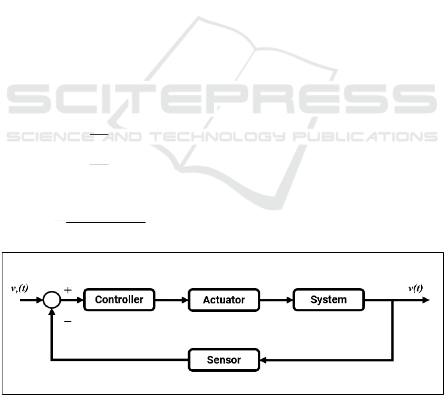
4 PROPORTIONAL INTEGRAL

DERIVATIVE LONGITUDINAL

CONTROLLER FOR SPEED

REGULATION

The input variables of the motorcycle model are the

steering angle and the driving torque at the rear

wheel. The steering angle assigned during the

simulation process, derives from experimental

acquisitions, whereas the driving torque input to

assign at the rear wheel has been evaluated through

the implementation of a Proportional-Integral-

Derivative (PID) controller, on the longitudinal

velocity.

The PID controller is a closed-loop control

system. It requires a sensor that is able to measure the

controlled variable and sends the corresponding

information to the controller. The controller receives

as input the error made on the controlled variable, i.e.

between the velocity signal and the target velocity;

based on that error and using a proper control law

evaluates the control signal to be sent to the actuator

that applies the control force on the system in such a

way the controlled variable follows the reference.

The PID controller generates an output that is

given by the summation of three different contribute

that are respectively proportional to the error between

the reference signal and the output signal, to its

derivative and to its integral over time.

Therefore, the driving torque input assumes the

following form:

v





−v





+k

v





−v







v





−v





dt

(14)

Figure 3: Closed loop control system - block diagram.

VEHITS 2021 - 7th International Conference on Vehicle Technology and Intelligent Transport Systems

296

5 ROLL ANGLE STABILIZATION

Motorcycle is an unstable system that is kept in the

stable zone by its rider that acts as a feedback

controller acting on throttle, brake, steer, roll and by

moving himself on the seat influencing the centre of

gravity position, so the forces and the torques acting.

Reproducing the driver's behaviour with a math

model has always been very tricky since there are

many variables that must be taken into consideration.

Furthermore, there is no optimal strategy to adopt due

to the fact that it depends on parameters related to the

riding style of a specific riders.

Defining an optimal strategy for the roll motion

control is a hard and complex thing. The usual

approach is to balance the bike and to put it in the

stable zone at the beginning; then, once it is stable,

the body movement is controlled to exploit the best

grip and speed. Many difficulties figure out on that

strategy, for example, the body cannot be considered

as a point mass but should at least be schematized like

a solid with homogeneously distributed weight. Since

this control part requires a lot of time to be tuned and

to be simulated, the approach used here starts from

the ideal roll angle.

The motorcycle, in steady turning, is subject to

both a restoring moment, generated by the centrifugal

force that tends to return the motorcycle to a vertical

position, and to a tilting moment, generated by the

weight force, that tends to increase the motorcycle’s

inclination or roll angle.

The following simplifying hypotheses have been

introduced:

▪ the motorcycle runs along a turn of constant

radius at constant velocity (steady-state

conditions);

▪ the gyroscopic effect is negligible.

Considering the cross-section thickness of the tires to

be zero, the moments equilibrium allows to derive the

roll angle φ in terms of the forward velocity V

and

the radius of the turn R

(measured from the centre of

gravity to the turning axis):

φ = tan

-1



= tan

-1





(15)

Where Ω indicates the angular yaw rate, while

V=ΩR

indicates the vehicle forward velocity.

In equilibrium conditions, the resultant of

centrifugal and weight forces passes through the line

joining the contact points of the tires on the road

plane. This line lies in the motorcycle plane if the

wheels have zero thickness and the steering angle is

very small.

Figure 4: Steady turning: roll angle equipped with zero

thickness tires (Cossalter, 2014).

In this work, therefore, to implement a control

system that allowed the roll angle stabilization for the

roll angle, the ideal roll angle is used as an input of

the model to ensure stability. The rider presence is

neglected, so no movement outside the plane of the

motorcycle is considered, but it has been assumed that

the rider rigidly attached to the saddle and always

remains in the plane of symmetry of the motorcycle.

Because of this assumption, the roll angle acquired by

experimental measures and the one derived by

imposing the steady turning conditions differ a bit

from each other.

6 RESULTS

The data obtained from the model have been

compared with those obtained from the experimental

acquisitions given by a high-performance motorcycle

manufacturing company; the industrial partner also

provide all the information necessary to parametrize

the model properly. The results have been then

normalized for reasons of confidentiality.

The model inputs are the steer angle and the rear

torque that were evaluated by the PID controller that,

on the error between the target velocity and the

measured velocity, applied a driving torque to the rear

wheel of the motorcycle. For this reason, the profile

velocity that is obtained is quite close to the velocity

acquired experimentally, as illustrated in Fig. 5.

Non-linear Motorcycle Dynamic Model for Stability and Handling Analysis with Roll Motion and Longitudinal Speed Regulation

297

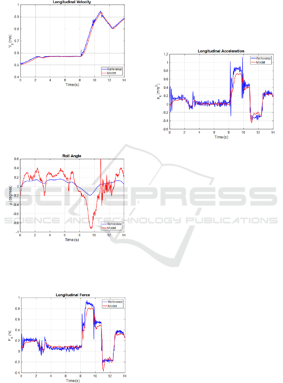
Figure 5: Velocity profile comparison.

It can be noticed that the roll angle of the model

is globally greater than that acquired experimentally

as expected since the rider is considered to be rigidly

attached to the saddle and can’t move his entire

bodies to the interior of the turn to reduce the roll

angle of the motorcycle.

Figure 6: Roll angle comparison.

Moreover, there is a good match on the

longitudinal force at the rear wheel and on the

longitudinal acceleration between the model and the

acquired data as shown in Fig. 7 and Fig. 8.

Figure 7: Longitudinal force comparison.

As it is possible to see in those figures, the model

replies longitudinal force and acceleration correctly

in all the dynamic conditions, except for the high

acceleration zones; this is mainly due to the

simplification introduced in the motorcycle

schematization and parametrization.

Figure 8: Longitudinal acceleration comparison.

7 CONCLUSIONS

In the present work, the mathematical model of a

motorcycle with four degrees of freedom has been

presented. The study has been carried out under the

hypotheses of considering the front wheel steering

and the rear wheel driving and braking. Any motion

of the rider has been neglected, therefore the roll

angle assigned during the simulation is equal to the

ideal roll angle evaluated for the steady-state

conditions. To simulate the behaviour of a driver who

tries to reach a certain velocity has been implemented

a proportional-integral-derivative controller PID

which according to the error between the target

velocity and the measured velocity apply a driving

torque to the rear wheel of the motorcycle. For tire

modelling, a physical model to describe the friction

forces between the tire/road interface has been

adopted, which is the Dugoff tire model.

The comparison has shown good reliability of the

proposed model especially for what concerns the

longitudinal dynamics, although have been found

some differences between the lateral forces due to the

basic hypotheses for the model of considering the

ideal roll angle and to neglect any dynamic due to the

rider behaviour.

The availability of non-linear equations

represents an advantage with respect to the classical

Jacobian linearization approach commonly used in

literature. The model can be employed with an

advanced non-linear model-based control system

VEHITS 2021 - 7th International Conference on Vehicle Technology and Intelligent Transport Systems

298

design and it can also be easily implemented on board

thanks to its simplicity and robustness.

Further developments may consist in the

realization of a more complex motorcycle model,

considering it as a multi-body system of four bodies:

the front and rear wheels, the rear assembly

(including frame, engine and fuel tank), the front

assembly (including steering column, handle-bar, and

front fork). Moreover, a suspension system at the

front and at the rear could also be considered; in this

way, it could be analyzed the degrees of freedom of

the motorcycle in the longitudinal plane such as the

pitch motion and the vertical displacement.

The model developed could also be completed

with a rider leaning model for the roll stabilization. In

particular, it could be implemented a rider control in

which the rider tries to stabilize the motorcycle by

inclining left and right his upper body in such a way

to not consider the roll angle fixed to its steady-state

value, in order to have a better description of

transverse dynamics.

REFERENCES

Bruni, S., Meijaard, J. P., Rill, G., Schwab, A. L., 2020.

State-of-the-art and challenges of railway and road

vehicle dynamics with multibody dynamics

approaches. Multibody System Dynamics, 49(1).

Cossalter, V., 2014. Motorcycle dynamics. Lulu.com.

Cossalter, V., Lot, R., 2002. A motorcycle multi-body

model for real time simulations based on the natural

coordinates approach. Vehicle System Dynamics, 37(6),

423–447.

Dugoff, H., Fancher, P. S., Segel, L., 1969. Tire

Performance Characteristics Affecting Vehicle

Response to Steering and Braking Control Inputs.

Escalona, J. L., Kłodowski, A., Muñoz, S., 2018. Validation

of multibody modeling and simulation using an

instrumented bicycle: from the computer to the road.

Multibody System Dynamics, 43(4), 297–319.

Escalona, J. L., Recuero, A. M., 2012. A bicycle model for

education in multibody dynamics and real-time

interactive simulation. Multibody System Dynamics,

27(3), 383–402.

Farroni, F., Russo, M., Sakhnevych, A., Timpone, F., 2019.

TRT EVO: Advances in real-time thermodynamic tire

modeling for vehicle dynamics simulations.

Proceedings of the Institution of Mechanical Engineers,

Part D: Journal of Automobile Engineering, 233(1),

121–135.

Farroni, F., Sakhnevych, A., Timpone, F., 2019. A three-

dimensional multibody tire model for research comfort

and handling analysis as a structural framework for a

multi-physical integrated system. Proceedings of the

Institution of Mechanical Engineers, Part D: Journal of

Automobile Engineering, 233(1), 136–146.

Genovese, A., Carputo, F., Maiorano, A., Timpone, F.,

Farroni, F., Sakhnevych, A., 2020. Study on the

Generalized Formulations with the Aim to Reproduce

the Viscoelastic Dynamic Behavior of Polymers.

Applied Sciences, 10(7), 2321.

Genovese, A., Farroni, F., Papangelo, A., Ciavarella, M.,

2019. A Discussion on Present Theories of Rubber

Friction, with Particular Reference to Different Possible

Choices of Arbitrary Roughness Cutoff Parameters.

Lubricants, 7(10), 85.

Genta, G., 1997. Motor Vehicle Dynamics. World Scientific

Publishing Co. Pte. Ltd.

Gillespie, T. D., 1996. Fundamentals of Vehicle Dynamics

- Thomas D.Gillespie (pp. 1–294).

Herlihy, D. V., 2004. Bicycle : the history. Yale University

Press.

Koenen, C., 1983. The dynamic behaviour of a motorcycle

when running straight ahead and when cornering.

Kooijman, J. D. G., Schwab, A. L., 2011. A review on

handling aspects in bicycle and motorcycle control.

Proceedings of the ASME Design Engineering

Technical Conference, 4(PARTS A AND B), 597–607.

Leonelli, L., Mancinelli, N., 2015. A multibody motorcycle

model with rigid-ring tyres: Formulation and

validation. Vehicle System Dynamics, 53(6), 775–797.

Limebeer, D. J. N., Sharp, R. S., Evangelou, S., 2002.

Motorcycle steering oscillations due to road profiling.

Journal of Applied Mechanics, Transactions ASME,

69(6), 724–739.

Lowell, J., McKell, H. D., 1982. The stability of bicycles.

American Journal of Physics, 50(12), 1106–1112.

Pacejka, H. B., & Sharp, R. S., 1991. Shear Force

Development by Pneumatic Tyres in Steady State

Conditions: A Review of Modelling Aspects. Vehicle

System Dynamics, 20(3–4), 121–175.

Pacejka, H. B., 2006. Tire and Vehicle Dynamics.

Rajput, B., Bayliss, M., Transactions, D. C.-S., 2007. A

simplified motorcycle model. JSTOR.

Romano, L., Sakhnevych, A., Strano, S., Timpone, F.,

2019. A hybrid tyre model for in-plane dynamics.

Vehicle System Dynamics, 1–23.

Sakai, H., 1990. Study on Cornering Properties of Tire and

Vehicle. Tire Science and Technology, 18(3), 136–169.

Schwab, A. L., Meijaard, J. P., Papadopoulos, J. M., 2004.

Benchmark Results on the Linearized Equations of

Motion of an Uncontrolled Bicycle.

Seffen, K. A., Parks, G. T., Clarkson, P. J., 2001.

Observations on the controllability of motion of two-

wheelers. Proceedings of the Institution of Mechanical

Engineers, Part I: Journal of Systems and Control

Engineering, 215(2), 143–156.

Sharp, R. S., 1971. The Stability and Control of

Motorcycles. Journal of Mechanical Engineering

Science, 13(5), 316–329.

Sharp, R. S., Alstead, C. J., 1980. The Influence of

Structural Flexibilities on the Straight-running Stability

of Motorcycles. Vehicle System Dynamics, 9(6), 327–

357.

Non-linear Motorcycle Dynamic Model for Stability and Handling Analysis with Roll Motion and Longitudinal Speed Regulation

299

Sharp, R. S., & Limebeer, D. J. N., 2001. A Motorcycle

Model for Stability and Control Analysis. Multibody

System Dynamics, 6(2), 123–142.

Spierings, P. T. J., 1981. The Effects of Lateral Front Fork

Flexibility on the Vibrational Modes of Straight-

Running Single-Track Vehicles. Vehicle System

Dynamics, 10(1), 21–35.

Yi, J., Zhang, Y., Song, D., 2009. Autonomous motorcycles

for agile maneuvers, Part I: Dynamic modeling.

Proceedings of the IEEE Conference on Decision and

Control, 4613–4618.

VEHITS 2021 - 7th International Conference on Vehicle Technology and Intelligent Transport Systems

300