
Trends Identification in Medical Care
In
ˆ
es Sena
a
and Ana I. Pereira
b
Research Centre in Digitalization and Intelligent Robotics (CeDRI), Instituto Polit
´
ecnico de Braganc¸a, Braganc¸a, Portugal
Keywords:
Artificial Intelligence, Machine Learning, Support Vector Machine, Classification Algorithm, Reliability.
Abstract:
Daily, health professionals are sought out by patients, motivated by the will to stay healthy, making numerous
diagnoses that can be wrong for several reasons. In order to reduce diagnostic errors, an application was devel-
oped to support health professionals, assisting them in the diagnosis, assigning a second diagnostic opinion.
The application, called ProSmartHealth, is based on intelligent algorithms to identify clusters and patterns
in human symptoms. ProSmartHealth uses the Support Vector Machine ranking algorithm to train and test
diagnostic suggestions. This work aims to study the application’s reliability, using two strategies. First, study
the influence of pre-processing data analysing the impact in the accuracy method when data is previously pro-
cessed. The second strategy aims to study the influence of the number of training data on the method precision.
This study concludes the use of pre-processing data and the number of training data influence the precision of
the model, improving the precision on 8%.
1 INTRODUCTION
Through the availability of data, the variety of data
analysis techniques and the information processing
capacity of computers, Artificial Intelligence, Ma-
chine Learning and Deep Learning have increasingly
contributed to the medical industry in different do-
mains and applications, enabling the creation of pre-
dictive models that allow the study of transmis-
sion and identification of disease risk, among others
(Academy, 2015), (Jiang et al., 2017).
This study consisted of developing an applica-
tion that provides diagnostic suggestions to support
health professionals in order to reduce diagnostic er-
rors. This application manages, for now, diagnoses of
three types of diseases: breast cancer, dementia and
heart disease.
The application, called ProSmartHealth, uses Su-
pervised Learning approach (Kim, 2017), through
classification strategy to identify the type of diag-
noses. ProSmartHealth uses Support Vector Machine
method with algorithms of linear binary classification
and multi-class approach.
Although ProSmartHealth obtained satisfactory
results, achieving a precision of 84%, there were
many aspects to improve. So, the application update
was done using two strategies: the influence of the
a
https://orcid.org/0000-0003-4995-4799
b
https://orcid.org/0000-0003-3803-2043
pre-processing data on the train set and the perfect
number of training data to obtain the best model ac-
curacy.
The paper is organised as follows: The section
2 presents a review of the literature on how Artifi-
cial Intelligence, Machine Learning and Support Vec-
tor Machine can be applied in the health field. The
3 section demonstrates the ProSmartHealth applica-
tion. The 4 section presents the problem to be devel-
oped and the 5 section presents a description of the
databases used. The numerical results will be pre-
sented and analysed in Section 6. Finally, Section 7
summarises the work with some conclusions and per-
spectives for future work.
2 LITERATURE REVIEW
Artificial Intelligence (AI) assists in several areas,
having already been implemented in several applica-
tions, namely in the autonomous car, on the factory
floor, in the hospital service system, in social net-
works, on the mobile phone, among others (Russel
and Norvig, 2004). The AI system can support doc-
tors by providing up-to-date medical information, in
addition, with a large number of information, it is pos-
sible to create software that warns of risk, or can di-
agnose and predict the onset of diseases (Miotto et al.,
2017).
Sena, I. and Pereira, A.
Trends Identification in Medical Care.
DOI: 10.5220/0010384502950302
In Proceedings of the 10th International Conference on Operations Research and Enterprise Systems (ICORES 2021), pages 295-302
ISBN: 978-989-758-485-5
Copyright
c
2021 by SCITEPRESS – Science and Technology Publications, Lda. All rights reserved
295

Machine Learning (ML) is used more often in
the health area, performing segmentation of medi-
cal images, named image registrations, image fusion,
computer-assisted diagnosis, image-guided therapy,
image annotation, and data set retrieval image (Khare
et al., 2017). An example of use is the development of
a model for a hospital classification based on a diag-
nosis of hospitalisations, with and without emergency,
where it is predict the urgency of admissions with a
numerical value that reflects the degree of planning
available for a hospital. This study helps to identify
the increasing emergency services in hospitals, which
can be a complex scheduling problem (Kr
¨
amer et al.,
2019).
Support Vector Machine (SVM) was already ap-
plied in healthcare by increasing diagnostic accuracy.
An example of use on the prediction of Alzheimer’s
disease, which has the final diagnosis provided with
the corresponding values. This training is carried out
through a binary classification method. In this study,
the algorithm was able to predict dementia and vali-
date its performance through statistical analysis (Bat-
tineni et al., 2019).
3 ProSmartHealth APPLICATION
The ProSmartHealth application consists in an intelli-
gent system to identify clusters and patterns in human
symptoms and aims to assist health professionals in
the diagnosis process, through an integrated question-
naire with key questions that the professional fills in
with patient data and obtains a diagnostic suggestion
(for now, three diseases are available: heart disease,
breast cancer and dementia).
This application was developed, in the Matlab
software, combining three model codes that provide
a diagnostic suggestion for each disease individually.
The application procedure started by studying which
is the best algorithm for the data set to be used through
Matlab Classification Learner application, obtaining
the best results from the Support Vector Machine.
To use this classification method, it is necessary
that the data set is divided into two sets: training and
testing. The training data set has 85% of the total nu-
merical data and the test data set has the remaining
15% of the numerical data. These data sets were used
to train and test the model in 100 iterations with the
appropriate algorithms for each data set, taking into
account that the Support Vector Machine algorithms
depend on the number of classes to be identified.
For breast cancer and heart disease, have two
classes, the fitcsvm function is used with the mini-
mum sequential optimisation algorithm, the function
implements the algorithm represented in Figure 1.
Figure 1: Linearly Separable Problem algorithm (N. Deng
and Zhang, 2013).
As dementia data has three classes, the fitcecoc func-
tion is used, which executes the “one vs one” method
with a linear kernel, the algorithm implemented by
the function can be seen in Figure 2.
Figure 2: One vs One method algorithm (N. Deng and
Zhang, 2013).
The three models codes were combined to cre-
ate the ProSmartHealth application. The application
starts with a home page where the health professional
can choose the disease to acquire a diagnostic sugges-
tion, as shown in Figure 3.
Depending on the disease chosen by the health
professional, a window will appear with a question-
naire that will have a number of questions representa-
tive of the parameters used to train and test the model,
in the case of breast cancer there are ten, for demen-
tia there are 5 and for heart disease there are thirteen
parameters, which are explained in Section 5.
When the health professional finishes filling out
the chosen questionnaire the system will send a mes-
sage indicating a diagnostic suggestion.
ICORES 2021 - 10th International Conference on Operations Research and Enterprise Systems
296

Figure 3: ProSmartHealth application home.
4 PROBLEM STATEMENT
Diagnostic errors are increasingly common in the
health area, which is beginning to worry the popu-
lation (dos Santos et al., 2010). These errors can oc-
cur in different sectors and for several reasons, one of
them is the fact that hospitals are often overcrowded
and without enough doctors to monitor 100% of all
patients.
Therefore, the ProSmartHealth application aims
to reduce diagnostic errors, assisting health profes-
sionals.
Given this, this study is based on the study of the
reliability of ProSmartHealth through two strategies.
The first strategy consists of studying the impact of
pre-processing data. The second strategy is based on
studying the influence of the number of training data
on the accuracy of the model.
5 DATA SET
CHARACTERISATION
For the application, it was necessary a data set in
which each data is formed by a set of input parameters
(characteristics) and a set of classes, which represent
the phenomenon of interest on which it is intended to
make predictions. So far, the application considers the
diagnosis associated with heart disease, breast cancer
and dementia.
This study used three different data sets, one for
each disease. The data set for breast cancer contains
569 data in 10 parameters were obtained from the
University of Wisconsin through an aspiration biopsy
(Qassim, 2018), dementia includes 150 data in 5 pa-
rameters acquired through the series of open access
imaging studies (Battineni et al., 2019), and heart dis-
ease covers 303 data in 14 parameters obtained by the
Cleveland data set (Latha and Jeeva, 2019).
Next, the different parameters of each disease that
characterise each database will be presented.
5.1 Breast Cancer
The data set consists of 357 patients who were diag-
nosed with a benign nodule and 212 patients were di-
agnosed with a malignant nodule. The ten input pa-
rameters and the used in this study were:
Radius: Calculated by averaging the distance from
the center to the perimeter points. This parameter
comprises values between 6.98 mm and 28.11 mm;
Texture: Calculated using the standard deviation of
the gray scale values. The values vary between 9.71
and 39.3;
Perimeter: Calculated through the distance from the
center to the perimeter points, diameter (d). The vari-
ation of values happens between 43.79 mm and 188.5
mm;
Area: Calculated using 2π × d. This parameter com-
prises values between 143.5 mm
2
and 2501 mm
2
;
Smoothness: Local variation in radius lengths. The
variation in the values of this parameter is included in
0.0526 and 1158;
Compression: It is calculated using
perimeter
2
/area − 1.0. The values vary between
0.0107 and 0.3;
Concavity: Severity of the concave portions of the
contour. The range of values for this parameter is be-
tween 0 and 0.5;
Concave: Measurement of the surface deeper in the
center than at the end. This parameter comprises val-
ues between 0 and 0.27;
Symmetry: Symmetry of the duct holes. This param-
eter comprises values between 0 and 0.3;
Fractal Dimension: Value of ”approaching the
coast”. The range of values for this parameter is be-
tween 0 and 1.2;
Diagnosis: This database obtains two possible diag-
noses, benign and malignant nodules, represented by
0 and 1, respectively.
5.2 Dementia
This data set comprises results from 150 different pa-
tients, where 77 of the patients are characterised as
non-demented, 58 of the individuals as demented, and
the remaining 15 as converts, that is, non-demented at
the time of their initial visit and subsequently char-
acterised as demented, on a later visit. The six input
parameters taken into account were as follows:
Trends Identification in Medical Care
297

Age: It is the main risk factor for diseases of the de-
mentia level. This parameter includes ages from 60 to
93 years old;
Clinical Dementia Rating (CDR): It is a tool for
studying dementia that classifies individuals with dis-
abilities in each of the seven domains: memory,
guidance, judgement and problem solving, function
in community affairs, home, hobbies and personal
care. Based on the collateral source and the patient
interview, a score is obtained if CDR = 0 without
Alzheimer’s, if CDR = 0.5 Very mild Alzheimer’s,
CDR = 1 Mild Alzheimer’s, CDR = 2 Moderate
Alzheimer’s;
Mini-Mental State Examination (MMSE): It is a
neuropsychological test that evaluates, from 0 to 30,
several abilities, such as reading, writing, orientation
and short-term memory. Thus, a score greater than 24
points indicates healthy cognitive performance, be-
tween 19 and 23 points corresponds to mild dementia,
between 10 and 18 points represents moderate demen-
tia and less than 9 points represents severe dementia;
MR Delay: It is the interval between each image re-
moved; This parameter comprises values that vary be-
tween 0 and 2639;
Normalized Whole-Brain Volume (n-WBV): is cal-
culated using an image that is initially segmented to
classify brain tissue as cerebral spinal fluid, gray or
white matter. The segmentation procedure iteratively
assigned voxels (matrix of volume elements that con-
stitute a three-dimensional space) to tissue classes.
The n-WBV is then calculated as the amount of all
voxels within each fabric class. This parameter com-
prises values that vary between 0.6 and 0.8;
Diagnosis: This database obtains three possible diag-
noses, non-demented, converted and demented, rep-
resented by 0, 1 and 2, respectively.
5.3 Heart Disease
The data set used in the Cleveland database consists
of a longitudinal collection of 303 patients, where 138
of the patients have no heart disease, and 165 of the
patients have heart disease. The fourteen input pa-
rameters used in this study were:
Age: The most important risk factor in the develop-
ment of heart disease, because blood pressure tends to
increase with age, this is due to the fact that blood ves-
sels have lost their elasticity. This parameter includes
ages from 29 to 77 years old;
Gender: Men are at higher risk for heart disease than
women in pre-menopause, but after menopause the
risk is similar to that of a man. In the database, 0
corresponds to women and 1 to men;
Angina (Chest Pain): Angina is chest pain or dis-
comfort caused when the heart muscle does not re-
ceive enough oxygen-rich blood. The type of chest
pain that the patient feels is displayed by: 1 (typical
angina), 2 (atypical angina), 3 (non-angina pain) and
4 (asymptotic);
Resting Blood Pressure: One of the risk factors, be-
cause high blood pressure can damage the arteries
that feed the heart, and the increase in blood pres-
sure inside the arteries also causes the heart to have to
greater effort to pump blood. The value is displayed
in mmHg, where the values for systolic (maximum)
vary between 120 mmHg and 180 mmHg and for di-
astolic (minimum) vary between 80 mmHg and 110
mmHg;
Cholesterol: Because a high level of low-density
lipoprotein (LDL) cholesterol is a risk factor for car-
diovascular disease. The value is represented in
mg/dl, which varies between 130 mg/dl and 50 mg/dl,
meaning very high cardiovascular risk and low car-
diovascular risk, respectively;
Fasting Blood Sugar: Not producing enough hor-
mone secreted by the pancreas (insulin) or not re-
sponding properly to insulin causes your body’s blood
sugar levels to rise, increasing the risk of a heart at-
tack. An individual’s fasting blood sugar value is
compared with 120 mg/dl, if the value is greater than
120 mg/dl, then it has a value of 1 (true) otherwise a
value of 0 (false);
ECG at Rest: Because it is an exam that detects the
electrical activity of the heart, being the most used
to assess cardiac arrhythmia’s. Displays results such
as: 0 (normal), 1 (with ST-T wave abnormality) and 2
(left ventricular hypertrophy);
Maximum Heart Rate Reached: increased cardio-
vascular risk is associated with accelerated heart rate.
The values vary between 60 bpm and 100 bpm, which
represent, low heart rate and high heart rate, respec-
tively;
Exercise-induced Angina: The pain or discomfort
associated with angina can vary from mild to severe,
with an affirmative value of 1 and negative if 0;
Exercise ST Segment Peak: An exercise test on the
ECG is considered abnormal when there is a horizon-
tal ST depression or downward slope ≥ 1 mm at 60-
80 ms after the J point. The parameter comprises val-
ues that vary between 0 and 6.2 mm;
Peak Exercise ST Segment: The duration of ST seg-
ment depression is also important, as prolonged re-
covery after peak stress is consistent with a positive
stress test on the ECG, can be represented in case of
climb by 1, in case of stability / plane by 2 and in case
of descent by 3;
Number of Main Vessels: From 0 to 4 which are col-
ICORES 2021 - 10th International Conference on Operations Research and Enterprise Systems
298
ored by fluoroscope, is displayed by an integer value;
Thalassemia: It is a group of inherited diseases
resulting from an imbalance in the production of
one of the four chains of amino acids that make up
hemoglobin, in 3 (normal), 6 (corrected defect) and 7
(reversible defect);
Diagnoses: This database obtains two possible diag-
noses, absence and present, represented by 0 and 1,
respectively.
6 RESULTS ANALYSIS
As already mentioned, the reliability of the applica-
tion was studied using two strategies: the first strategy
is to measure the impact of the pre-processing data,
and the second is based on the study of the influence
of the number of training data on the accuracy of the
response.
In the first strategy, the data set is pre-processed,
by cleaning the data set, removing all outliers found.
Then the precision of the model is calculated for the
data set with pre-processing, through the same proce-
dure, being compared with the precision obtained for
the original data set.
The second strategy is based on studying the in-
fluence of the number of training data on the model’s
accuracy. In which the accuracy of the model with
10k cross-validation will be calculated for three dif-
ferent training sets, one with 85% (performed in the
previous strategy), another with 75% and finally 65%.
The results are obtained for both data sets, with and
without pre-processing of the data, to verify whether
these factors matter for the calculation of the model’s
precision.
It is necessary to bear in mind that the test data
set is always the same for all attempts so that the re-
sults are reliable. In the following section, these two
strategies were carried out for each disease studied,
analysing each result, referring at the end to the im-
provements that this study brought to the application.
6.1 Breast Cancer
As mentioned in Section 5.1, the original breast can-
cer data set consists of 569 data, of which 357 belong
to the benign class and 212 to the malignant class.
For the first strategy, the boxplot technique was
used to remove all outliers from the database, in
which 107 outliers of the benign class and 40 outliers
of the malignant class were identified and removed,
so the treated data set contains 422 data.
Subsequently, the prediction of the model was cal-
culated using the data set treated using the procedure
referred to in Section 3, where the set was divided into
a training set with 85% of the numerical data (359)
and a set of test with 15% of numerical data (63).
Then the precision obtained for the original and
treated data set was compared, which can be seen in
Table 1.
Table 1: Comparison of precision values.
Original data set Treated data set
Precision 84.71% 98.41%
By analysing Table 1, it can be indicated that the
model’s accuracy improves when the data set is pre-
processed, even if only the outliers have been re-
moved.
In order to observe the improvements in the preci-
sion of the model, the confusion matrices were com-
pared for each data set, analysing whether the percent-
age of false negatives and positives decreases with the
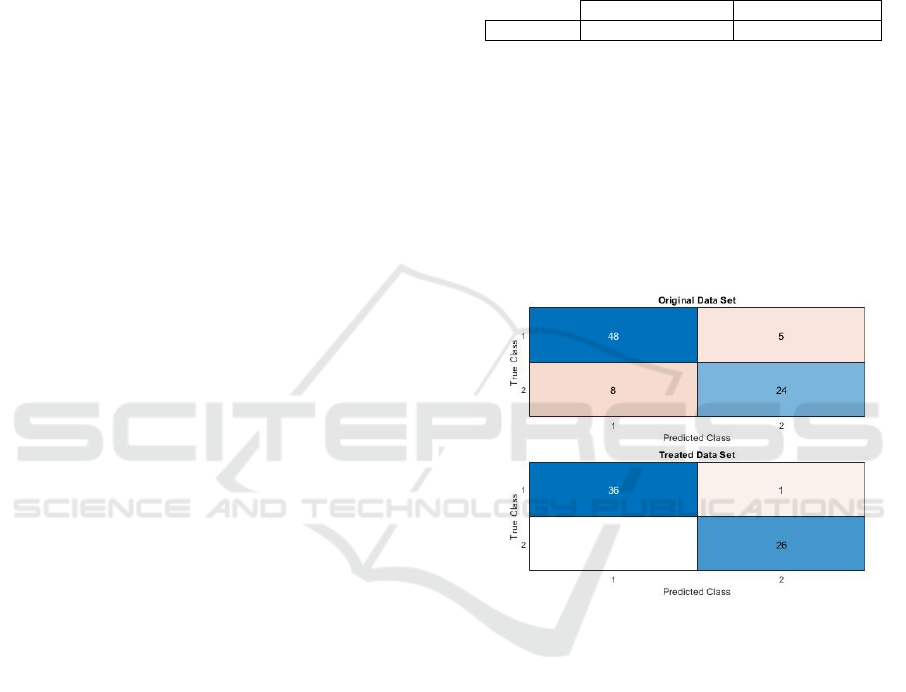
use of the treated data set. Figure 4 shows the confu-
sion matrices for each data set.
Figure 4: Comparison of confusion matrix.
Through Figure 4 it is possible to calculate the per-
centage of false negatives and positives for each set of
data used. For the original data set, 56.47% true pos-
itives, 28.24% true negatives, 9.41% false negatives
and 5.88% false positives were obtained. And, for the
treated data set, 57.14% true positives, 41.27% true
negatives, 1.59% false positives and 0.00% false neg-
atives were obtained. These results indicate that when
using a treated data set it is possible to obtain better
results, in this case it is clear that with the cleaning of
the data set, no false positive diagnosis is obtained.
Then, the second strategy was performed, in
which the model precision was calculated for each
data set with 75% and 65% of the data in a 10k cross-
validation, the test data are the same as those used
in the first strategy (15%) for each data set. Table 2
intends to compare the model’s precision values ob-
tained.
Trends Identification in Medical Care
299
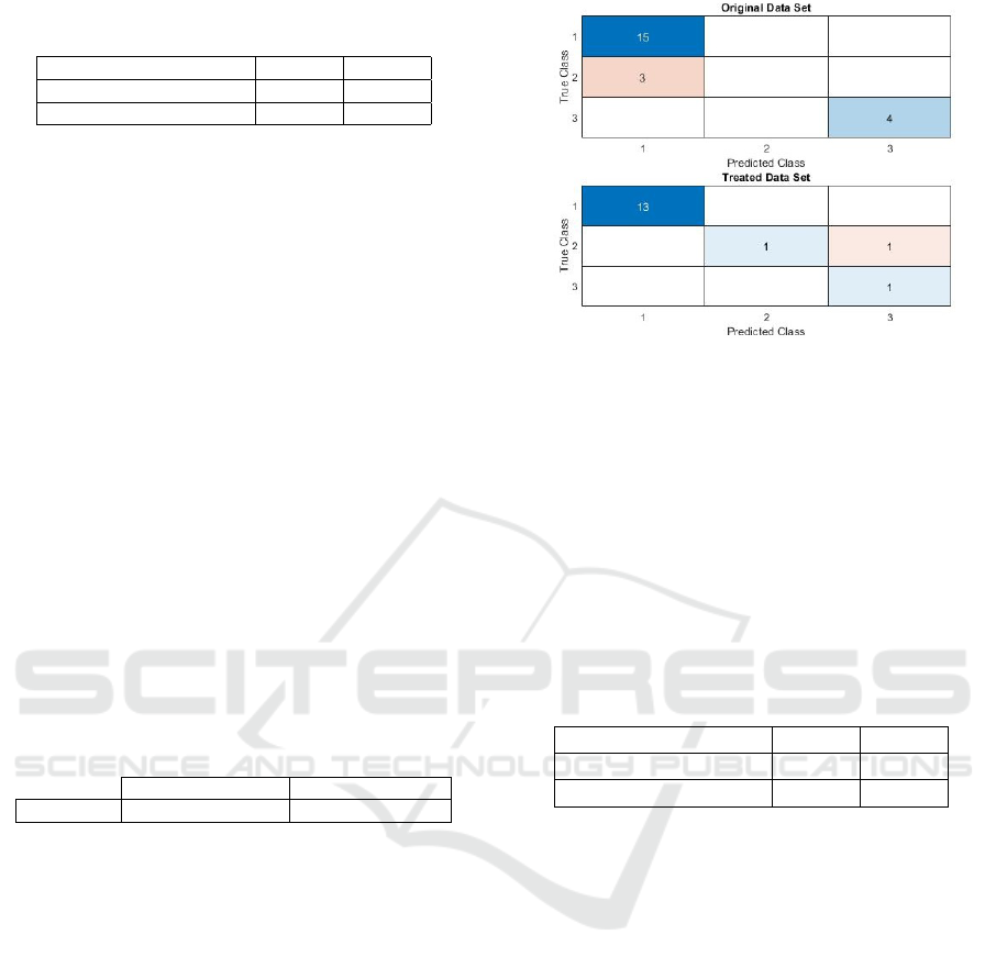
Table 2: Precision comparison with different numbers of
training data.
Training percentage 75% 65%
Original Data set 86.71% 85.88%
Pre-processed Data set 96.99% 96.51%
When checking the precision results of both Ta-
bles, 1 and 2, one can compare whether the precision
value decreases from 85% to 65% for each data set.
Then it can be indicated that through the treated data
set this happens, which is usually correct, because the
smaller the number of data to be used, the precision
should decrease because there is less data to train the
model.
6.2 Dementia
As mentioned in Section 5.2, the dementia data set
consists of 150 data, and through the boxplot tech-
nique it was observed that there were 9 outliers of the
non-demented class, 5 of the converted and 29 of the
demented, thus the treated data set contains 107 data.
To calculate the accuracy of the model with the
treated data set, it was divided into two sets: training
set with 91 numerical data (85%) and test set with 16
numerical data (15%).
Then, in Table 3, it is possible to observe the com-
parison of precision between the original data set and
the treated one.
Table 3: Comparison of precision values.
Original data set Treated data set
Precision 86.36% 93.75%
By analysing the Table 3 it is possible to indicate
that when performing the pre-processing of the data,
even if it is only the removal of the outliers, the accu-
racy of the model increases.
In order to better observe the differences between
the obtained precision, the confusion matrix was cre-
ated for each data set. Their comparison can be seen
in Figure 5.
Through the confusion matrices observed in Fig-
ure 5 it is possible to calculate various percentages
and check if there have been improvements in them
for each data set. For the original data set 68.18% true
positives, 18.18% true negatives and 6.82% false neg-
atives and 6.82% false positives were obtained, and
for the treated data set, the following percentages of
results are obtained: 81.25% true positives, 6.25%
true negatives and 6.25% false negatives and 6.25%
false positives.
With these results it can be indicated that there is
an improvement in the results when using the treated
data set, however, there is a lower percentage of true
Figure 5: Comparison of confusion matrix.
negatives that can be justified through the use of fewer
test data representative of the demented class, because
there are fewer test data set and data are chosen at
random.
Then, the second strategy is performed, which
consists of calculating the model precision for each
data set with a different number of training data in a
10k cross-validation, although the test data for each
set are the same as those used in the first strategy. Ta-
ble 4 shows the comparison of these results.
Table 4: Precision comparison with different numbers of
training data.
Training percentage 75% 65%
Original Data set 86.36% 86.36%
Pre-processed Data set 91.25% 87.50%
Using Table 3 and 4, it can be indicated that for the
treated data set, the precision decreases as the number
of data used to train the model decreases, the same is
not the case for the original data set. This may indi-
cate that the treated data set is more reliable.
6.3 Heart Disease
As mentioned in the 5.3 section, the original heart dis-
ease data set consists of 303 data, and in the first strat-
egy, the data were pre-processed by removing out-
liers, where 47 outliers were found. absence class
and 36 of the presence class, the data set being treated
with 220 data.
To calculate the accuracy of the model with the
treated data set, it is necessary to divide it into two
sets: training and testing. The training set contains
85% of the numerical data (187) and the test set con-
tains the remaining 15% of the numerical data (33).
It should be noted that the precision of the model was
calculated using the same process referred to in Sec-
tion 3 for the original data set.
ICORES 2021 - 10th International Conference on Operations Research and Enterprise Systems
300
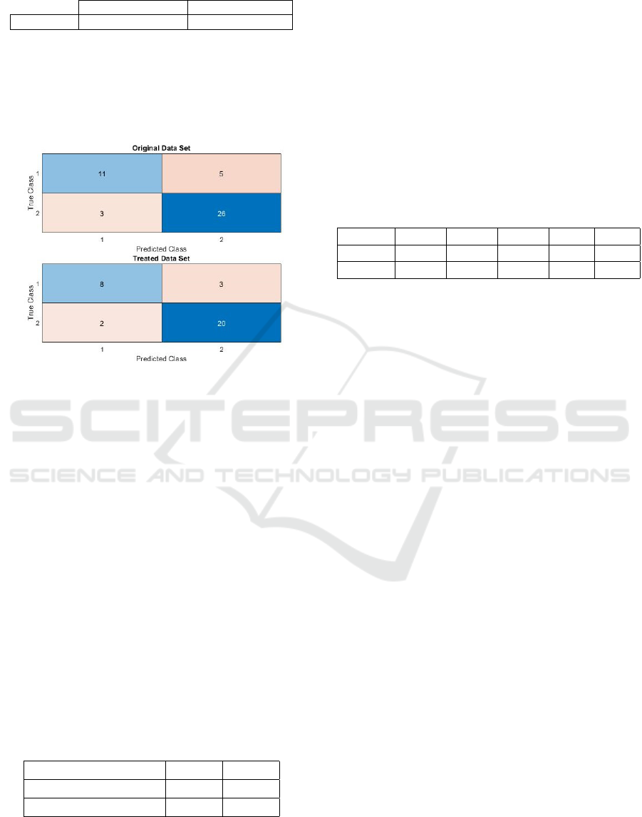
Table 5: Comparison of precision values.
Original data set Treated data set
Precision 82.22% 84.85%
Through Table 7 it is possible to observe that with
the use of the treated data set the precision of the
model increased. However, to verify this increase,
a confusion matrix was created and compared with
the one calculated for the original data set. Figure 6
shows the two confusion matrices.
Figure 6: Comparison of confusion matrix.
With Figure 6 it is possible to calculate various
percentages that demonstrate the reason for the in-
crease in precision between the treated and original
data set. 57.78% true negatives, 24.44% true posi-
tives, 11.11% false positives and 6.67% false nega-
tives were obtained for the original data set, and for
the treated data set, if 60.60% true negatives, 24.24%
true positives, 9.09% false negatives and 6.06% false
positives. Analysing these results, it can be indicated
that there was an improvement in the results when us-
ing a treated data set.
Then the second strategy was carried out, which
aims to study the influence of the number of training
data on the calculation of accuracy. Accuracy is cal-
culated for two more cases, 75% and 65% of the train-
ing data, maintaining the test sets used in the previous
strategy for each data set. Table 6 presents the com-
parison of the precision results of each data set for
each case.
Table 6: Precision comparison with different numbers of
training data.
Training percentage 75% 65%
Original Data set 82.00% 82.66%
Pre-processed Data set 84.55% 83.34%
When analysing the Table 4 and 6, it can be seen
that for the data set treated, the precision of the model
decreases as the percentage of numerical data used to
train the model decreases, which does not happen for
the original data set. This strategy demonstrates that
both the number of training data to be used and the
pre-processing of data influences the accuracy of the
model.
Table 7 shows the comparison between the orig-
inal and treated data set for the results obtained for
the ProSmartHealth application. Where is indicated
the total precision obtained by the application (Prec.),
The percentage of true positives (TP), true negatives
(TN), false negatives (FN) and false positives (FP).
Table 7: Precision comparison of ProSmartHealth applica-
tion.
Data Set Prec. TP TN FN FP
Original 84.00% 49.70% 34.73% 7.63% 7.94%
Treated 92.34% 54.21% 36.04% 4.63% 5.11%
Through Table 7 it is possible to observe that there
was an evolution in the results with the use of the
treated data sets. Where the accuracy of the model
has increased and the percentage of data predicted in-
correctly has decreased.
7 CONCLUSIONS AND FUTURE
WORK
Support Vector Machine is a good solution for the
medical industry, supporting numerous sectors in the
area, and in this case, by diagnosing patients early, it
is possible to support healthcare professionals to re-
duce errors in diagnosis, reducing the hospital stress.
It can be concluded that the pre-processing and
the number of training data influence the model ac-
curacy. There is an improvement in the results in the
three databases, where breast cancer data achieves the
best results, obtaining a very pleasant model precision
and containing minimum percentages of false posi-
tives and negatives.
In general, it is concluded that using a data set
with data pre-processing improves the precision of the
application by 8% in relation to the data sets without
pre-processing. Therefore, it can be stated, through
this study, that the pre-processing of the data and the
number of training data that is used to train the model
influence its accuracy.
Considering all this reliability analysis, the ProS-
martHealth application was updated with databases
with pre-processing, changing to ProSmartHealth 2.0,
an improved application with better results precision.
However, there are still many aspects to improve, such
as being applied to a greater number of diseases, and
Trends Identification in Medical Care
301

further decreasing the likelihood of obtaining false di-
agnoses.
Referring that the ProSmartHealth 2.0 application
was not developed with the intention of replacing
health professionals, but rather helping them, with
some alerts.
In the future, the ProSmartHealth 2.0 application
may be applied to a set of data with symptoms that
covers a greater number of diseases, which will allow
a suggestion of diagnosis with the percentage of con-
tracts each of these diseases that can be observed with
the data entered in the questionnaire.
ACKNOWLEDGEMENTS
This work has been supported by FCT — Fundac¸
˜
ao
para a Ci
ˆ
encia e Tecnologia within the Project Scope:
UIDB/05757/2020.
REFERENCES
Academy, D. S. (2015). Deep learning book.
http://deeplearningbook.com.br/uma-breve-historia-
das-redes-neurais-artificiais/. Online; accessed: 01
April 2020.
Battineni, G., Chintalapudi, N., and Amenta, F. (2019).
Machine learning in medicine: Performance calcu-
lation of dementia prediction by support vector ma-
chine (svm). Informatics in Medicine Unlocked,
(16):100–200.
dos Santos, M. C., Grilo, A., Andrade, G., Guimar
˜
aes, T.,
and Gomes, A. (2010). Comunicac¸
˜
ao em sa
´
ude e a
seguranc¸a do doente: problemas e desafio. Revista
Portuguesa de sa
´
ude p
´
ublica, 10:43–57.
Jiang, F., Jiang, Y., Zhi, H., Dong, Y., Li, H., Ma, S., Wang,
Y., Dong, Q., Shen, H., and Wang, Y. (2017). Arti-
ficial intelligence in healthcare: past, present and fu-
ture. Stroke and Vascular Neurology, 27(2):97–111.
Khare, A., Jeon, M., Sethi, I. K., and Xu, B. (2017). Ma-
chine learning theory and applications for healthcare.
Journal of Healthcare Engineering, page 2.
Kim, P. (2017). Matlab, Deep Learning – With Machine
Learning, Neural Networks and Artificial Intelligence.
Apress, London, 2nd edition.
Kr
¨
amer, J., Schrey
¨
ogg, J., and Bussel, R. (2019). Classifica-
tion of hospital admissions into emergency and elec-
tive care: a machine learning approach. Health Care
Manag Sci, (22):85–105.
Latha, C. B. C. and Jeeva, S. C. (2019). Improving the
accuracy of prediction of heart disease risk based on
ensemble classificarion techniques. Informatics in
Medicine Unlocked, (16):1–9.
Miotto, R., Wang, F., Wang, S., Jiang, X., and Dudley, J. T.
(2017). Deep learning for healthcare: Review, oppor-
tunities and challenges. Briefings in Bioinformatics,
6(19):1236–1246.
N. Deng, Y. T. and Zhang, C. (2013). Support Vector Ma-
chine - Optimization Based Theory, Algorithms, and
Extensions. Chapman & Hall Book/CRC Press, Min-
neapolis.
Qassim, A. (2018). Breast cancer cell type classi-
fier. https://towardsdatascience.com/breast-cancer-
cell-type-classifier-ace4e82f9a79. Online; accessed:
03 May 2020.
Russel, S. and Norvig, P. (2004). Intelig
ˆ
encia Artificial: Un
Enfoque Moderno. Pearson Educaci
´
on, S.A, London,
2nd edition.
ICORES 2021 - 10th International Conference on Operations Research and Enterprise Systems
302
