
Driving Behavior Analysis and Traffic Improvement using Onboard
Sensor Data and Geographic Information
Jun-Zhi Zhang and Huei-Yung Lin
a
Department of Electrical Engineering, National Chung Cheng University, Chiayi 621, Taiwan
Keywords:
Driving Behavior Analysis, Geographic Information System, Data Mining.
Abstract:
In this paper, we present a method to extract the training and testing data from geographic information system
(GIS) and global position system (GPS) for neural networks. Traffic signs, traffic lights and road information
from the OpenStreetMap (OSM) and the government platform are compared with driving data and videos
to extract images containing the important information. We also propose traffic improvement suggestions
for intersections or roads by analyzing the relationship between driving behaviors, traffic lights, and road
infrastructures. We use OBD-II and CAN bus logger to record more driving information, such as engine speed,
vehicle speed, steering wheel steering angle, etc. We analyze the driving behavior using sparse automatic
encoders and data exploration to detect abnormal and aggressive behavior. The relationship between the
aggressive driving behavior and road facilities is derived by regression analysis, and some suggestions are
provided for improving specific intersections or roads.
1 INTRODUCTION
In recent years, the field of self-driving cars has be-
come more and more popular. Many companies and
research institutes have started the development of au-
tonomous vehicle systems. It is very likely to have
self-driving cars and the vehicles controlled by human
drivers co-exist on the road in the future. In this re-
gard, one of the key components to the success of self-
driving systems is to understand the human driving
behavior in order to avoid the human-machine con-
flict (Dong and Lin, 2021). With the recent advances
of machine learning techniques, the data-driven ap-
proaches have made the complicated human behavior
modeling move a big step forward. Especially, some
researches with significant progress have been con-
ducted using deep learning (Hartford et al., 2016).
For the modern learning approaches, in addition to
the design of network structures, another major issue
is the requirement of a large amount of training data.
In the automative applications, this usually involves
the data collection from on-board sensors and the in-
formation extraction for specific analysis purposes.
These might include the images captured by the in-
car cameras for environment perception, and the pro-
prioceptive driving data recorded by the on-board di-
agnostics systems. In either case, it is necessary to
a
https://orcid.org/0000-0002-6476-6625
extract proper data segments for neural network train-
ing and testing. For instance, learning the road sign
recognition uses certain traffic scene images, or mod-
eling the driver’s acceleration behavior uses selected
gas pedal information. The use of large datasets for
training is commonly agreed for deep neural networks
to perform well or better.
In the early stage of related research, data annota-
tion or labeling are mostly done manually, and some-
times through crowdsourcing such as using Amazon
Mechanical Turk. For driving images, the dataset col-
lected according to different tasks contains a variety
of scenes and features. Since the selection and fil-
tering of adequate data require significant time and
human labor, it motivates a data management prob-
lem: How to search specific traffic scenes within a
large amount of image sequences? In this work, we
present a road scene extraction system for specific
landmarks and indicators of the transportation infras-
tructure. The information derived from GIS (geo-
graphic information system) and GPS are used with
the recorded driving videos to identify the road scenes
with static objects such as traffic lights, traffic signs,
bridge and tunnel, etc.
On the other hand, in addition to the exterocep-
tive sensors (such as LiDAR, GPS, camera, etc.), the
information collected from prioceptive sensors of the
vehicle can also be used to analyze the driving behav-
284
Zhang, J. and Lin, H.
Driving Behavior Analysis and Traffic Improvement using Onboard Sensor Data and Geographic Information.
DOI: 10.5220/0010384102840291
In Proceedings of the 7th International Conference on Vehicle Technology and Intelligent Transport Systems (VEHITS 2021), pages 284-291
ISBN: 978-989-758-513-5
Copyright
c
2021 by SCITEPRESS – Science and Technology Publications, Lda. All rights reserved

ior (Yeh et al., 2019). The sensor data derived directly
from the vehicle operation can provide more compre-
hensive driving information. It allows the researchers
and practitioners to study driving behaviors and traffic
safety issues more precisely. In this paper, we adopt
OBD-II (on-board diagnostics) and CAN bus (Con-
troller Area Network) logger to collect data. By mea-
suring a number of parameters at high sampling rate,
it is possible to fully observe the driving behaviors in
real life, and understand how they are affected by the
traffic and road infrastructures.
To analyze the relationship between the driving
behavior and the transportation infrastructure, its vi-
sualization on the map provides a way for better ob-
servation and investigation. We use machine learning-
based methods to extract the unique features from the
driving data and then map to the RGB color space to
visualize the driving behavior. The data mining algo-
rithms are adopted for data analysis and classify the
driving behavior into four categories, from normal to
aggressive. A regression analysis is then conducted
on the relationship between the aggressive driving be-
havior and the road features of intersections.
2 RELATED WORK
2.1 Training and Testing Data
Extraction
Due to the popularity of learning based algorithms in
recent years, the acquisition of training and testing
data has become an important problem. The current
data extraction approaches are mainly divided into
two categories, information-based and image-based
extraction. Hornauer et al. and Wu et al. (Hornauer
et al., 2019; Wu et al., 2018) proposed unsupervised
image classification methods to extract to the images
similarly to those provided by general users (Zhirong
et al., 2018). In supervised classification, the data are
labeled manually. People need to have similar under-
standing to annotate the same scene. Their network
presents a concept based on feature similarity for first-
person driving image query. However, it is not satis-
factory for the requests of most users.
In addition to the image extraction and classifi-
cation, Naito et al. developed a browsing and re-
trieval system for driving data analysis (Naito et al.,
2010). The system provides a multi-data browser, a
retrieval function based on query and similarity, and
a quick browsing function to skip extra scenes. For
the scene retrieval, the top N images highly similar
to the currently driving scenario are retrieved from
the database. In this technique, while the image se-
quence is processed, the system calculates the simi-
larity between the input scene and the scenes stored
in the database. A pre-defined threshold is used to
identify the similarity between the images. Since the
method mainly searches the driving video itself, it is
not able to know if the images contain the objects or
information interested to the users for precise extrac-
tion.
2.2 Driving Behavior Analysis
In the past few years, the key technologies of automa-
tive driving assistance systems have become more
mature (Lin et al., 2020). However, the ‘autonomous’
vehicles are still not ready without the human drivers.
Due to the current limitations of driving assistance
systems, researchers and developers are seeking for
the solutions to enhance the human driving capability.
Since the driving habits are very difficult to change, it
is expected to have a human-centered driving environ-
ment to avoid dangerous situations. By understand-
ing the relationship among the traffic lights, road in-
frastructure and driving behavior, some transportation
improvement suggestions can be provided. Besides,
knowing the human reaction is also a crucial issue in
the future world with mixed human drivers and self-
driving cars.
For driving behavior analysis, Liu et al. proposed
a method using various types of sensors connected to
the control area network (Liu et al., 2014; Liu et al.,
2017). A deep sparse autoencoder is then used to ex-
tract the hidden features from driving data to visualize
the driving behavior. Alternatively, Constantinescu et
al. used both PCA and HCA methods to analyze the
driving data (Constantinescu et al., 2010). The perfor-
mance of the algorithms is verified by classifying the
driving behavior into six categories according to dif-
ferent aggressiveness. In the study of Kharrazi et al.,
the driving behavior is classified into three categories,
calm, normal and aggressive, by a method using quar-
tile and Kmeans (Kharrazi et al., 2019). The analysis
has demonstrated that Kmeans is able to provide good
driving behavior classification results.
In the above methods, the correlation between the
driving behavior and the environment is not investi-
gated. For the discussion of more specific events, Tay
et al. used the regression model to associate driv-
ing accidents with the environment (Tay et al., 2008).
Wong et al. used a negative binomial regression to
analyze the number of driving accidents and the road
features of the intersection (Wong, 2019). It can help
us understand the relationship between the accidents
and road features. The road intersection can also be
Driving Behavior Analysis and Traffic Improvement using Onboard Sensor Data and Geographic Information
285
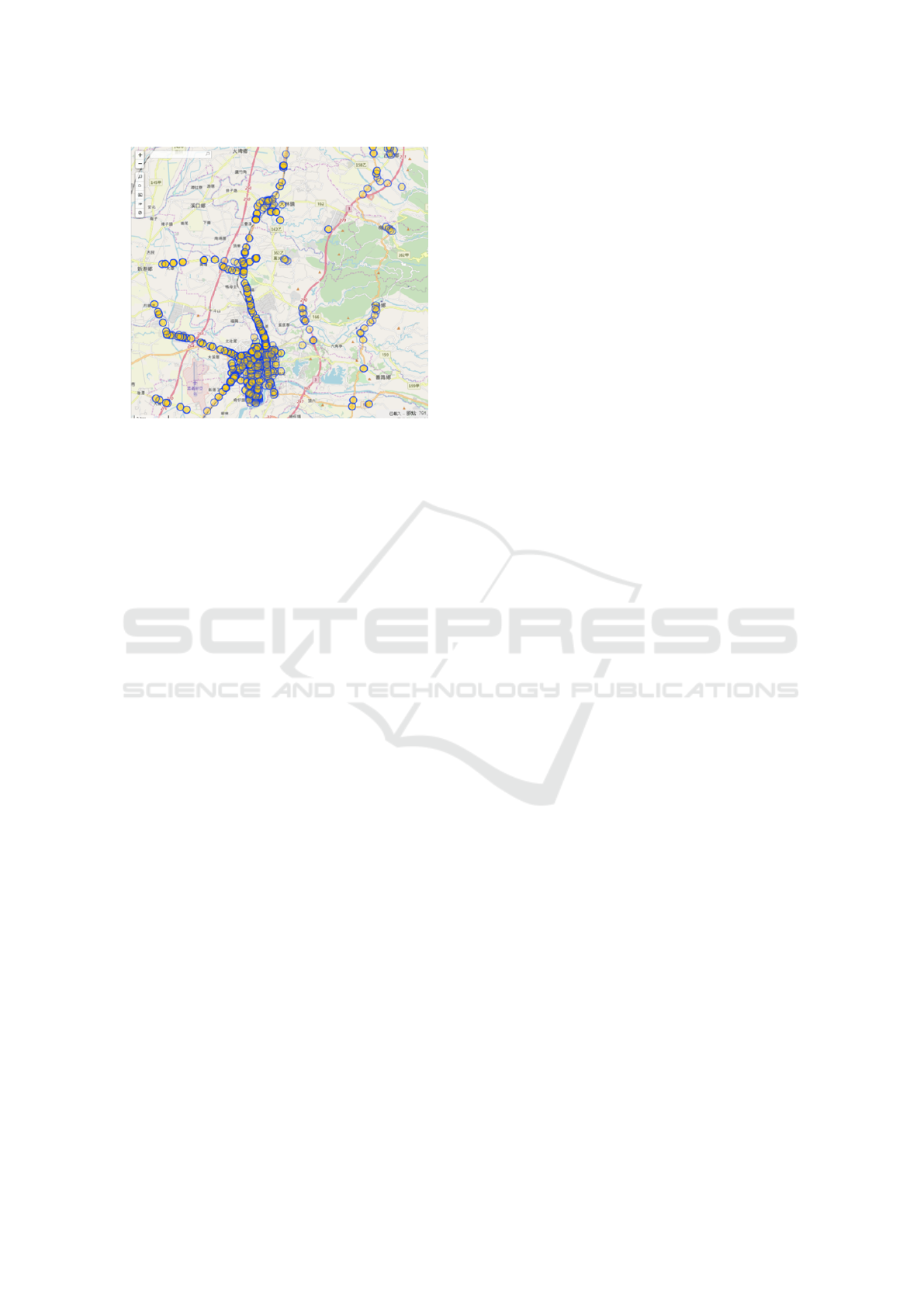
Figure 1: The traffic light information shown on the Open-
StreetMap. The yellow dots indicate the locations of traffic
lights on main roads.
improved by the simulation carried out based on the
analysis results. Schorr et al. recorded the driving
data in one and two-way lanes (Schorr et al., 2016).
Based on ANOVA analysis, the conclusion about the
impact of the lane width to the driving behavior is
drawn. Mohammad et al. investigated how the acci-
dents were affected specific driving behaviors through
a number of questionnaires and interviews (Aboja-
radeh et al., 2014). They used regression analysis
to derive the correlation between the number of ac-
cidents and the types of dangerous driving behaviors.
Regarding the improvement on transportation in-
frastructures, various suggestions were proposed for
different designs of roads and intersections. Chunhui
et al. proposed to optimize the signal lights at the
intersections to make the pedestrian crossing easier
(Chunhui et al., 2017; Wang et al., 2019). The ef-
ficiency of intersections is improved by reducing the
conflicts between the turning vehicles and pedestri-
ans. Ma et al. proposed to add a dedicated left-turn
lane and left turn waiting area according to the aver-
age daily traffic volume at the intersection (Ma et al.,
2017). The proposed method is able to accommodate
more vehicles waiting for left turn. They also an-
alyze three common left-turn operation scenarios at
the intersections and compare their differences. In
addition to the suggestions for road infrastructures,
there also exist some improvements based on the traf-
fic light analysis. In the recent work, Anjana et al.
presented a method based on different traffic volumes
at the intersections to evaluate the safety caused by the
green time of the traffic light (Anjana and Anjaneyulu,
2015).
3 DATASET EXTRACTION
We first collect traffic lights, traffic signs and road in-
formation on the OpenStreetMap (OSM) and the gov-
ernment’s GIS-T transportation geographic informa-
tion storage platform of the as the locations of inter-
est for image data extraction. Figure 1 illustrates an
example of the traffic light information shown on the
OSM. The yellow dots indicate the locations of traffic
lights on main roads. For image data extraction, the
transportation infrastructure and road information are
used to identify the locations of interest using the GPS
coordinates. We compare the GPS information of the
driving data and the locations of interest. The asso-
ciated images are then extracted and stored in video
sequences for specific application uses (such as the
training and testing data for traffic light detection).
The specifications of the driving recorder contain
the images with the resolution of 1280 ×720 and 110
◦
FOV (field-of-view) in the horizontal direction. To
extract the suitable image data, the users need to con-
sider a geographic range of the interested target. As
a typical example of road scene extraction with traffic
lights, the size of the traffic signal in the image might
be larger than 25 × 25 pixels for specific tasks. This
corresponds to about 50 meters away from the vehi-
cle, so the video should be pushed back 5 seconds to
start the image extraction.
A program interface is created for users to eas-
ily operate the data and assign the parameters. As
shown in Figure 2, it consists of folder selection, item
menu for extraction, OSM map display and driving
image screen. The user first select the folder where
the driving record video and driving GPS information
are located, and the folder where the extracted image
will be stored, followed by the selection of the traffic
infrastructure or road information to be extracted. On
the interface, the vehicle’s GPS trajectory and the user
selected traffic infrastructures simultaneously overlay
on the OSM window, and the synchronized driving
video is displayed on the right for inspection.
4 DRIVING BEHAVIOR
ANALYSIS
In this paper, we mainly focus on the analysis of driv-
ing behavior and the correlation with traffic and road
features. The common relationship is first established
and the studies on specific scenarios are then carried
out. The driving behavior is classified into normal and
aggressive, and analyzed through data visualization
and the regression model on the number of aggressive
driving behaviors and road features.
VEHITS 2021 - 7th International Conference on Vehicle Technology and Intelligent Transport Systems
286
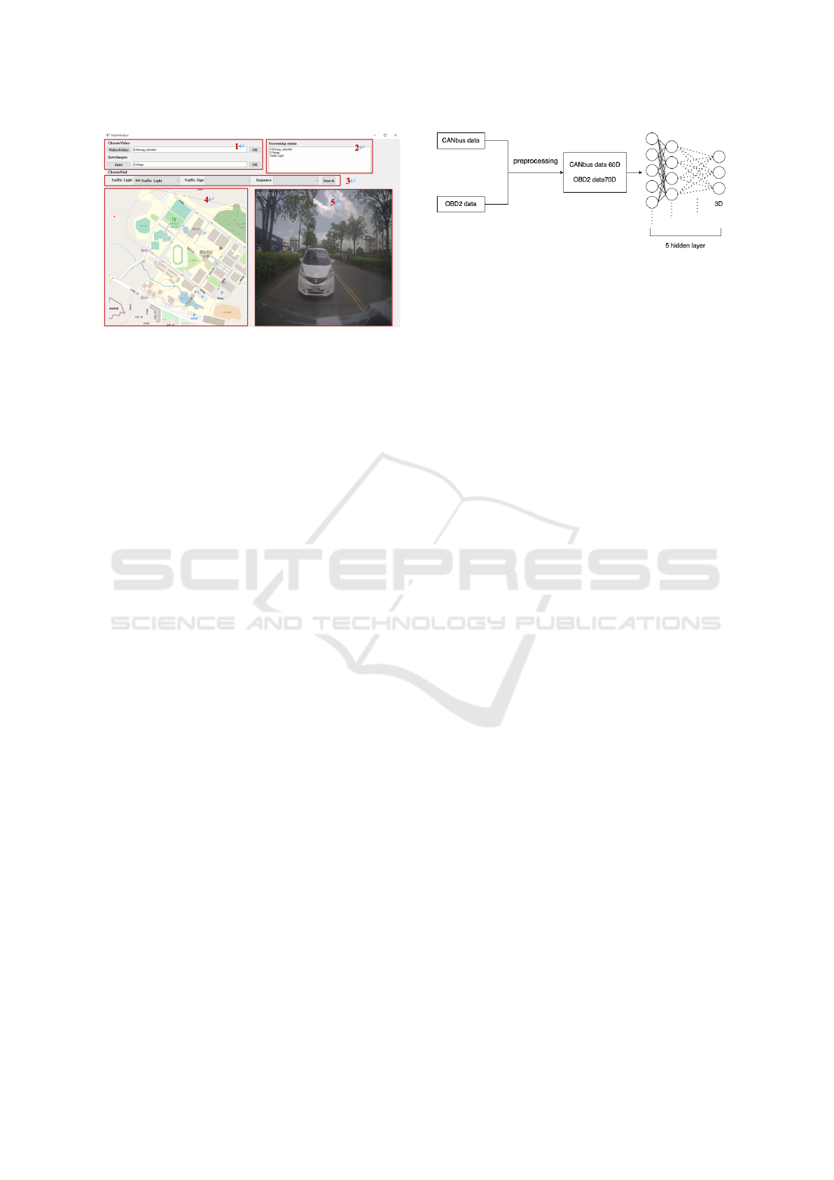
Figure 2: The user interface for image data extraction. 1.
folder selection, 2. processing status display, 3. extraction
item menu, 4. driving trajectory display, and 5. driving
video display.
4.1 Data Collection
The tools for data collection in this work include
ODB-II (Malekian et al., 2014) and CANbus loggers.
Unlike most previous work which only use the infor-
mation obtained from GPS receivers (with GPS mes-
sages, vehicle speed and acceleration), OBD-II and
CANbus loggers are able to collect various types of
driving data to analyze in more details. The specific
data types used for our driving behavior analysis are
as follows:
• OBD-II: engine rotating speed, engine load, throt-
tle pedal position, acceleration XYZ, and vehicle
speed.
• CANbus logger: engine rotating speed, throttle
pedal position, braking pedal position, steering
angle, wheel speed, and vehicle speed.
• GPS receiver: GPS and UTC.
In addition, we also use two public datasets, DDD17
dataset (Binas et al., 2017) and UAH Drive-set
(Romera et al., 2016). The datasets are acquired by
the driving monitoring application, DriveSafe, and
mainly used to verify the classification and analysis
methods (Bergasa et al., 2014).
4.2 Visualization of Driving Behavior
The relationship between the driving behavior and
traffic infrastructures can be observed by the data vi-
sualization on the map. We use the sparse autoen-
coder (SAE) to extract features from the driving data,
compress the high-dimensional features into three di-
mensions, and mapping to RGB space for display on
the OpenStreetMap (Liu et al., 2017). The loss func-
Figure 3: The flowchart and network structure for driving
behavior analysis.
tion with sparse constraints is given by
J
sparse
(W, b) = J (W, b) + β
s
2
∑
j=1
KL(ρ k
ˆ
ρ
j
) (1)
The difference between SAE and autoencoder (AE) is
that a penalty term is added to the loss function, so
the activation of the hidden nodes drops to the value
we need. Using this property, the relative entropy is
added to the loss function to penalize the value of the
average activation degree far away from the level ρ.
The parameters can keep the average activation de-
gree of hidden nodes at the level. Thus, the loss func-
tion only needs to add the penalty term of relative en-
tropy without sparse constraints.
Figure 3 illustrates the structure to visualize the
driving behavior. The network contains 9 hidden lay-
ers, and the dimensionality reduction of each layer is
half the number of nodes in the previous layer. Our
data collected by OBD-II contain 7 types, and become
70 dimensions after windowing process. Thus, the di-
mension reduction in the network is 70 → 35 → 17 →
8 → 3 → 8 → 17 → 35 → 70, and the features are
extracted by the last 5 layers. The data collected by
CANbus logger contain 6 types, and are processed to
60 dimensions after windowing. Likewise, the input
to the network consists of 60 nodes, and the dimen-
sion reduction is given by 60 → 30 → 15 → 7 → 3 →
7 → 15 → 30 → 60. Finally, the driving behavior is
visualized on the OpenStreetMap.
We use the Kmeans clustering algorithm to fur-
ther classify the driving behavior. The elbow method
is used to find the most appropriate k value to clas-
sify the driving behavior according to different ag-
gressiveness (Thorndike, 1953). From normal to ag-
gressive, it is classified into four levels, and the most
aggressive driving behavior is marked on the OSM.
4.3 Negative Binomial Regression
We refer to (Wong, 2019) and use negative binomial
regression model to analyze the road features at in-
tersections and interchanges. It is an extended ver-
sion of Poisson regression to deal with the data over-
dispersed problem. The negative binomial regression
Driving Behavior Analysis and Traffic Improvement using Onboard Sensor Data and Geographic Information
287
model
µ
i
= exp(β
1
x
1i
+ β
2
x
2i
+ ··· + β
k
x
ki
+ ε
i
) (2)
is used to predict the number of aggressive driving
behavior µ
i
, where β is the correlation term associated
with each road feature parameter, and ε
i
is an error
term. Next, we need to verify if the data are over-
dispersed, so Pearson’s chi-squared test is carried out
(Pearson, 1900). When the ratio is greater than 1, the
data is considered to be over-dispersed.
To evaluate whether the Poisson regression or
negative binomial regression can better fit our data,
Akaike information criterion (AIC) is calculated for
these two models (Akaike, 1974). AIC is an effec-
tiveness measure of data fitting on regression models
given by
AIC = 2k − 2ln(L) (3)
where k is the number of features and ln(L) is the
maximum likelihood. A smaller AIC value implies be
a better fitting model. As an example case, the max-
imum likelihoods of Poisson and negative binomial
regression are -21.457 and -21.758 respectively, and
the AIC values are 58.914 and 59.516 respectively.
It shows that the negative binomial regression model
has a smaller AIC. Thus, it is used as the model for
our analysis.
After classifying the driving behavior by Kmeans,
it is found that the aggressive driving behavior occurs
more frequently at the interchanges and intersections.
The negative binomial regression analysis is carried
out on these two specific driving scenarios. We adopt
the road features proposed by Wong (Wong, 2019)
and those commonly appeared in Taiwan road scenes
as follows.
1. Interchange: (1) section length, (2) lane width, (3)
speed limit, (4) traffic flow.
2. 4-Arm Intersection: (1) without lane marking, (2)
straight lane marking, (3) left lane marking, (4)
right lane marking, (5) shared lane marking, (6)
shared lane marking at roadside, (7) motorcycle
priority, (8) branch road.
3. 3-Arm Intersection: (1) without lane marking, (2)
straight lane marking, (3) shared lane marking at
roadside, (4) lane ratio, (5) motorcycle priority,
(6) branch road.
5 EXPERIMENTS
The experiments contain two parts: One is the system
for the extraction of training and testing dataset, and
the other is the driving behavior analysis based on the
driving and road features.
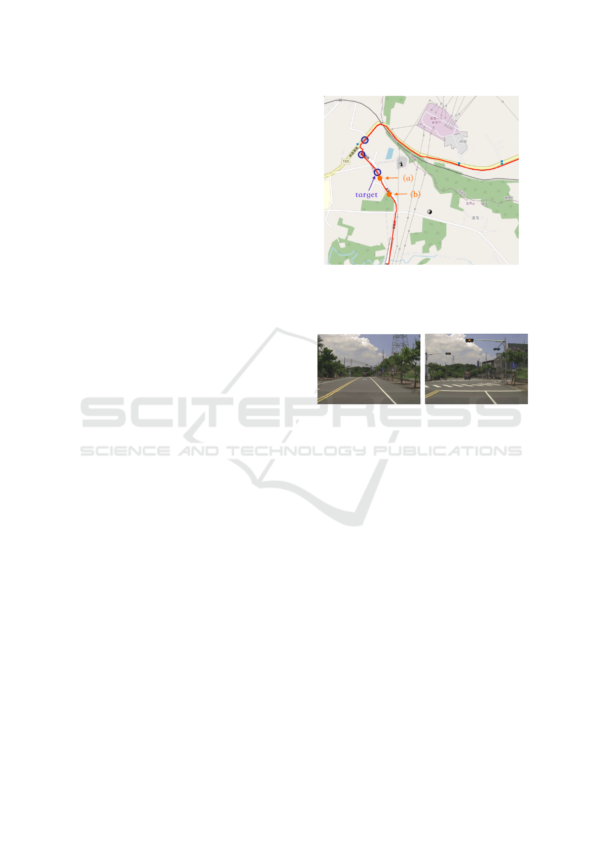
Figure 4: The driving trajectory (marked in red curve) and
traffic light positions (marked in purple circles) displayed
on the OpenStreetMap. The orange dots (a) and (b) corre-
spond to the images shown in Figures 5(a) and 5(b), respec-
tively.
(a) Long range image. (b) Short range image.
Figure 5: The images containing traffic lights extracted
from the map in 4, corresponding to the locations (a) and
(b), respectively.
5.1 Extraction of Training and Testing
Data
In this experiment, we demonstrate the image data ex-
traction for the road scenes with traffic lights. Fig-
ure 4 shows the driving trajectory (marked in red
curve) and traffic light positions (marked in purple
circles) displayed on OSM. The driving video is fil-
tered through the extraction system to contain the traf-
fic lights from the far to near distance. The extracted
images as shown in Figures 5(a) and 5(b) correspond
to the orange dots (a) and (b) on the map (in Figure
4), respectively.
5.2 Driving Behavior Analysis
For driving behavior analysis, the visualization and
Kmeans classification are presented first, followed by
the analysis on the driving behavior and road features.
VEHITS 2021 - 7th International Conference on Vehicle Technology and Intelligent Transport Systems
288
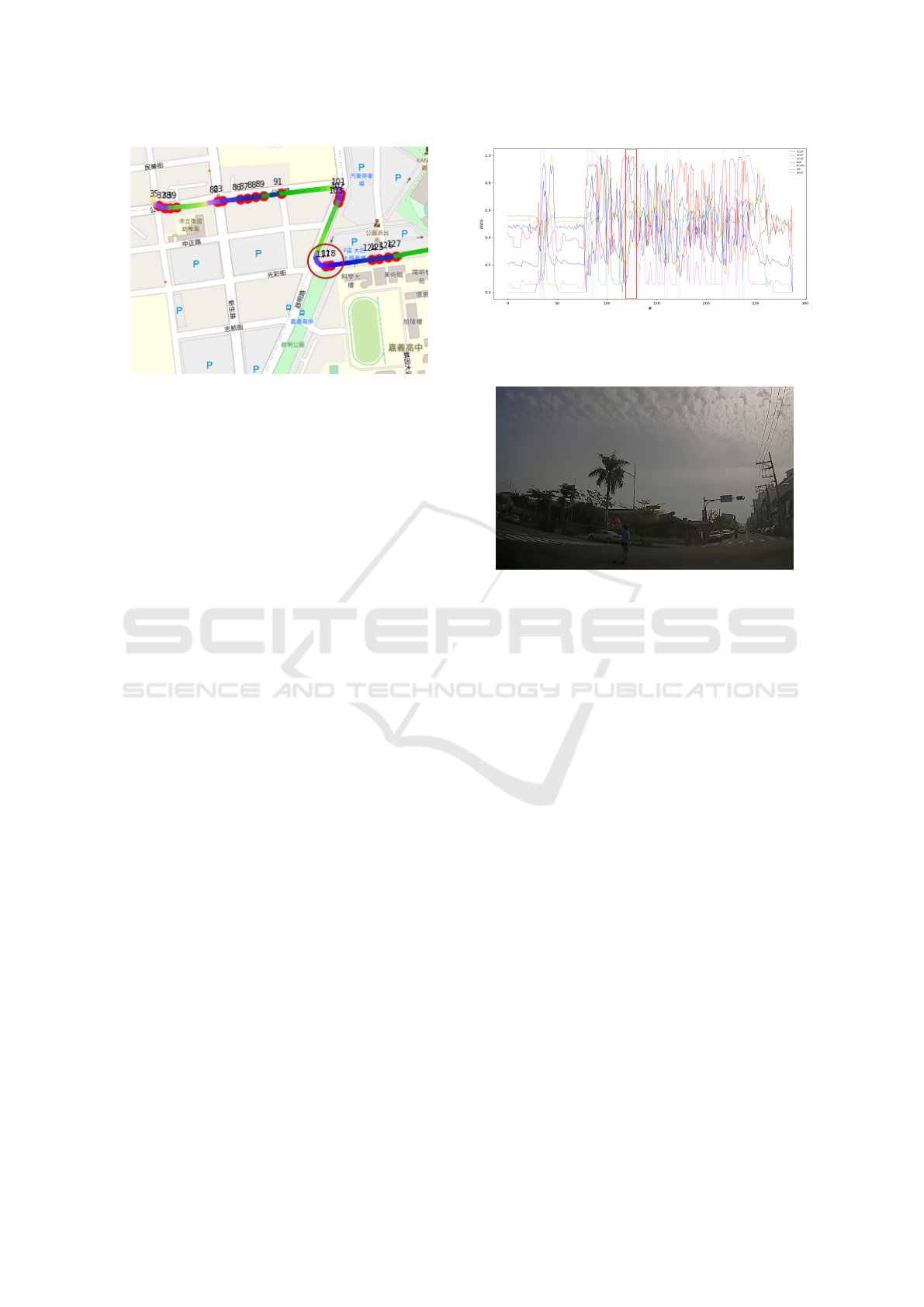
Figure 6: The visualized driving behavior. The aggres-
sive driving data and traffic lights are marked on the Open-
StreetMap. The red circle location corresponds to the data
enclosed by red in Figure 7 and the driving image shown in
Figure 8.
5.2.1 Visualization and Kmeans Classification
In this experiment, whether Kmeans can effectively
classify the driving behavior is verified first. We
use five segments of driving data in UAH Drive-set,
and the drivers are in normal and aggressive behav-
iors separately. In each data segment, 50 samples
are taken for classification. The results are shown in
Table 1 with the percentage of correct classification,
where D1 – D5 represent five drivers. N and A are
the normal and aggressive driving, respectively. The
table illustrates that Kmeans is able to provide satis-
factory classification results on normal and aggressive
driving behaviors.
Figure 6 shows the driving behavior (including ag-
gressive driving) using the driving data collected by
ourselves visualized on OpenStreetMap with the traf-
fic light location information. The driving data chart
and the image acquired by a car digital video recorder
are shown in Figures 7 and 8, respectively. By ob-
serving the information from these three aspects, the
correlation among them can be analyzed. In this ex-
ample, the aggressive driving behavior at location in-
dicated by the red circle (Figure 6) is caused by a
pedestrian passing through the intersection (Figure 8),
which leads to the braking and turning of the vehicle
(Figure 7).
By visualizing the driving behavior and displaying
the aggressive driving behaviors on OSM with refer-
ence to the driving video, we are able to observe the
correlation between the driving behavior and traffic
infrastructure. Three situations are analyzed as fol-
lows.
a. The influence of two-way lanes on the driving be-
havior: We found that the vehicle speed in a two-
way lane is higher than a one-way lane. Thus,
Figure 7: The driving data chart. The red frame corresponds
to the location indicated by the red circle in Figure 6 and the
driving image in Figure 8.
Figure 8: The image acquired at the location corresponding
to the circle in Figure 6. A pedestrian passing through the
intersection leads the braking of the vehicle as illustrated in
Figure 7.
the aggressive driving behaviors with fast driving
and emergency braking are more likely to occur
in two-way lanes.
b. The influence of traffic lights on the driving be-
havior: We found that most of the aggressive driv-
ing behaviors occurred at intersections. There
might be many reasons, such as fast changing sig-
nals and the poor design of the road. These gener-
ally cause more conflicts between the drivers and
other vehicles.
c. The influence of interchanges on the driving be-
havior: In the highway traffic, we found that most
of the aggressive driving behaviors occur at inter-
changes. A vehicle entering the entrance of the
interchange tends to drive into the inner lane. This
generally causes the other drivers to change lanes
or slow down.
5.2.2 Negative Binomial Regression
Since the aggressive driving behaviors frequently oc-
cur near the intersections and interchanges, we further
investigate these driving scenarios using negative bi-
nomial regression analysis on the correlation between
the number of aggressive behaviors and road features.
Driving Behavior Analysis and Traffic Improvement using Onboard Sensor Data and Geographic Information
289
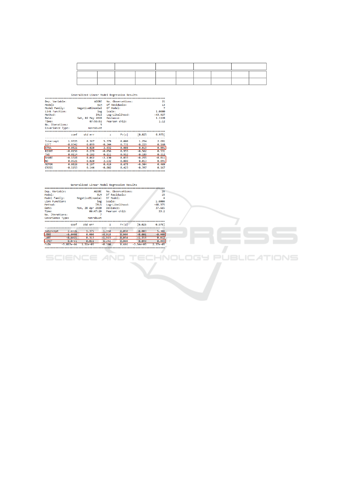
Table 1: The Kmeans classification performance on UAH Drive-set.
D1 D2 D3 D4 D5
N A N A N A N A N A
100% 80% 100% 100% 100% 96% 98% 100% 98% 98%
(a) The regression result at a 4-arms intersection.
(b) The regression result at a highway interchange.
Figure 9: The negative binomial regression analysis results
for a 4-arm intersection and a highway interchange. (a) In-
tercept: the error term of regression model, LEFT: left turn
lane mark, STRA: straight lane mark, RIGHT: right turn
lane mark, TWO: shared lane mark, SHARE: shared lane
mark on the side of the road, NO: no lane mark, MOTOR:
the number of priority locomotive lanes, CROSS: the num-
ber of branch roads and the coefficient term is the param-
eter by the regression model. (b) LONG: the length of in-
terchange, LANE: the width of the lane, LIMIT: the ramp
speed limit, and FLOW: the average daily traffic volume.
The P-value is used to evaluate whether the feature
has a significant impact on aggressive driving behav-
ior (Dahiru, 2008). Two driving scenarios are exam-
ined as follows.
4-Arms Intersection: There are eight different road
features at the intersections as defined previ-
ously. After the regression analysis as shown in
Figure9(a), we see the features that have great im-
pacts on the aggressive driving behaviors include
‘straight lane marking’, ‘shared lane marking at
roadside’ and ‘without lane marking’. The influ-
ences of these features on the driving behaviors
are positive correlation, negative correlation and
positive correlation, respectively. When “P > |z|”
< 0.05, the feature is important affects the aggres-
sive behavior.
Highway Interchange: There are four different road
features defined for the highway. After the regres-
sion analysis as shown in Figure 9(b), we see the
features that have great impacts on the aggressive
driving behaviors are ‘speed limit’ and ‘length of
interchange’. The influences of these features on
the driving behaviors are positive correlation and
negative correlation, respectively.
6 CONCLUSIONS
This paper presents the image data extraction based
on geographic information and driving behavior anal-
ysis using various types of driving data. The traffic in-
frastructure and GPS information are used to extract
specific road scenes for network training and testing
purposes. We use OBD-II and CANbus loggers to
acquire driving data, and classify the driving behav-
iors using SAE feature extraction and Kmeans algo-
rithm. The negative binomial regression analysis is
performed for specific scenarios. Our result show that
lane ratios, without lane markings, and straight lane
markings are important features which affect the ag-
gressive driving behavior. In the end, we present the
traffic improvements based on the analysis for a case
study at an intersection.
ACKNOWLEDGMENTS
This work was financially/partially supported by Cre-
ate Electronic Optical Co., LTD, Taiwan.
REFERENCES
Abojaradeh, M., Jrew, B., and Al-Ababsah, H. (2014). The
effect of driver behavior mistakes on traffic safety.
Journal of Civil and Envivornment Research, 6:39–
54.
Akaike, H. (1974). A new look at the statistical model iden-
tification. IEEE Transactions on Automatic Control,
19:716—-723.
VEHITS 2021 - 7th International Conference on Vehicle Technology and Intelligent Transport Systems
290

Anjana, S. and Anjaneyulu, M. (2015). Safety analysis
of urban signalized intersections under mixed traffic.
Journal of Safety Research, 52:9–14.
Bergasa, L. M., Almer
´
ıa, D., Almaz
´
an, J., Yebes, J. J., and
Arroyo, R. (2014). Drivesafe: an app for alerting inat-
tentive drivers and scoring driving behaviors. IEEE
Intelligent Vehicles Symposium(IV), pages 240–245.
Binas, J., Neil, D., Liu, S.-C., and Delbruck, T. (2017).
Ddd17: End-to-end davis driving dataset. Workshop
on Machine Learning for Autonomous Vehicles, pages
1–9.
Chunhui, Y., Wanjing, M., Ke, H., and Xiaoguang, Y.
(2017). Optimization of vehicle and pedestrian sig-
nals at isolated intersections. Transportation Research
Part B: Methodological, 98(C):135–153.
Constantinescu, Z., Marinoiu, C., and Vladoiu, M. (2010).
Driving style analysis using data mining techniques.
International Journal of Computers and Communica-
tions and Control, 5(5):654–663.
Dahiru, T. (2008). P-value, a true test of statistical signifi-
cance? a cautionary note. Annals of Ibadan Postgrad-
uate Medicine, 6:21—-26.
Dong, B. T. and Lin, H. Y. (2021). An on-board monitoring
system for driving fatigue and distraction detection.
In 2021 IEEE International Conference on Industrial
Technology, Valencia, Spain. (ICIT 2021).
Hartford, J. S., Wright, J. R., and Leyton-Brown, K. (2016).
Deep learning for predicting human strategic behav-
ior. In Lee, D. D., Sugiyama, M., Luxburg, U. V.,
Guyon, I., and Garnett, R., editors, Advances in Neu-
ral Information Processing Systems 29, pages 2424–
2432. Curran Associates, Inc.
Hornauer, S., Yellapragada, B., Ranjbar, A., and Yu, S.
(2019). Driving scene retrieval by example from
large-scale data. In Proceedings of the IEEE/CVF
Conference on Computer Vision and Pattern Recog-
nition (CVPR) Workshops.
Kharrazi, S., Frisk, E., and Nielsen, L. (2019). Driving
behavior categorization and models for generation of
mission-based driving cycles. IEEE Intelligent Trans-
portation Systems Conference, pages 1349–1354.
Lin, H. Y., Dai, J. M., Wu, L. T., and Chen, L. Q. (2020).
A vision based driver assistance system with for-
ward collision and overtaking detection. Sensors,
20(18):100–109.
Liu, H., Taniguchi, T., Takano, T., Tanaka, Y., Takenaka,
K., and Bando, T. (2014). Visualization of driving
behavior using deep sparse autoencoder. pages 1427–
1434.
Liu, H., Taniguchi, T., Tanaka, Y., Takenaka, K., and Bando,
T. (2017). Visualization of driving behavior based
on hidden feature extraction by using deep learning.
IEEE Transactions on Intelligent Transportation Sys-
tems, 18(9):2477–2489.
Ma, W., Liu, Y., jing Zhao, and Wu, N. (2017). Increasing
the capacity of signalized intersections with left-turn
waiting areas. Transportation Research Part A: Policy
and Practice, 105:181–196.
Malekian, R., Moloisane, N. R., Nair, L., Maharaj, B., and
Chude-Okonkwo, U. A. (2014). Design and imple-
mentation of a wireless obd ii fleet management sys-
tem. IEEE Sensors Journal, 13:1154–1164.
Naito, M., Miyajima, C., Nishino, T., Kitaoka, N., and
Takeda, K. (2010). A browsing and retrieval system
for driving data. IEEE Intelligent Vehicles Symposium,
pages 1159–1165.
Pearson, K. (1900). X. on the criterion that a given sys-
tem of deviations from the probable in the case of a
correlated system of variables is such that it can be
reasonably supposed to have arisen from random sam-
pling. The London, Edinburgh and Dublin Philosophi-
cal Magazine and Journal of Science, pages 157–175.
Romera, E., Bergasa, L. M., and Arroyo, R. (2016). Need
data for driver behaviour analysis? presenting the pub-
lic uah-driveset. International Conference on Intelli-
gent Transportation Systems (ITSC), pages 387–392.
Schorr, J., Hamdar, S. H., and Silverstein, C. (2016). Mea-
suring the safety impact of road infrastructure systems
on driver behavior: Vehicle instrumentation and ex-
ploratory analysis. Journal of Intelligent Transporta-
tion Systems.
Tay, Richard, Rifaat, Shakil, Chin, and Hoong (2008). A lo-
gistic model of the effects of roadway, environmental,
vehicle, crash and driver characteristics on hit-and-run
crashes. Accident; analysis and prevention, 40:1330–
6.
Thorndike, R. L. (1953). Who belongs in the family? Psy-
chometrika, 18(4):267–276.
Wang, Y., Qian, C., Liu, D., and Hua, J. (2019). Research on
pedestrian traffic safety improvement methods at typ-
ical intersection. 2019 4th International Conference
on Electromechanical Control Technology and Trans-
portation (ICECTT), pages 190–193.
Wong, C. K. (2019). Designs for safer signal-controlled
intersections by statistical analysis of accident data at
accident blacksites. IEEE Access, 7:111302–111314.
Wu, Z., Xiong, Y., Yu, S. X., and Lin, D. (2018). Unsu-
pervised feature learning via non-parametric instance
discrimination. 2018 IEEE/CVF Conference on Com-
puter Vision and Pattern Recognition, pages 3733–
3742.
Yeh, T. W., Lin, S. Y., Lin, H. Y., Chan, S. W., Lin, C. T.,
and Lin, Y. Y. (2019). Traffic light detection using
convolutional neural networks and lidar data. In 2019
International Symposium on Intelligent Signal Pro-
cessing and Communication Systems (ISPACS), pages
1–2.
Zhirong, W., A, E. A., and Stella, Y. (2018). Improving
generalization via scalable neighborhood component
analysis. European Conference on Computer Vision
(ECCV) 2018.
Driving Behavior Analysis and Traffic Improvement using Onboard Sensor Data and Geographic Information
291
