
Interpretability in Word Sense Disambiguation using Tsetlin Machine
Rohan Kumar Yadav, Lei Jiao, Ole-Christoffer Granmo and Morten Goodwin
Centre for Artificial Intelligence Research, University of Agder, Grimstad, Norway
Keywords:
Tsetlin Machine, Word Sense Disambiguation, Interpretability.
Abstract:
Word Sense Disambiguation (WSD) is a longstanding unresolved task in Natural Language Processing. The
challenge lies in the fact that words with the same spelling can have completely different senses, sometimes
depending on subtle characteristics of the context. A weakness of the state-of-the-art supervised models, how-
ever, is that it can be difficult to interpret them, making it harder to check if they capture senses accurately or
not. In this paper, we introduce a novel Tsetlin Machine (TM) based supervised model that distinguishes word
senses by means of conjunctive clauses. The clauses are formulated based on contextual cues, represented in
propositional logic. Our experiments on CoarseWSD-balanced dataset indicate that the learned word senses
can be relatively effortlessly interpreted by analyzing the converged model of the TM. Additionally, the clas-
sification accuracy is higher than that of FastText-Base and similar to that of FastText-CommonCrawl.
1 INTRODUCTION
Word Sense Disambiguation (WSD) is one of
the unsolved task in Natural Language Process-
ing (NLP) (Agirre and Edmonds, 2007) with rapidly
increasing importance, particularly due to the ad-
vent of chatbots. WSD consists of distinguishing the
meaning of homographs – identically spelled words
whose sense or meaning depends on the surrounding
context words in a sentence or a paragraph. WSD is
one of the main NLP tasks that still revolves around
the perfect solution of sense classification and indica-
tion (Navigli et al., 2017), and it usually fails to be in-
tegrated into NLP applications (de Lacalle and Agirre,
2015). Many supervised approaches attempt to solve
the WSD problem by training a model on sense anno-
tated data (Liao et al., 2010). However, most of them
fail to produce interpretable models. Because word
senses can be radically different depending on the
context, interpretation errors can have adverse con-
sequences in real applications, such as chatbots. It
is therefore crucial for a WSD model to be easily in-
terpretable for human beings, by showing the signifi-
cance of context words for WSD.
NLP is one of the discipline that are used as the
application in a chatbot. With the recent prolifera-
tion of chatbots, the limitations of the state-of-the-
art WSD has become increasingly apparent. In real-
life operation, chatbots are notoriously poor in distin-
guishing the meaning of words with multiple senses,
distinct for different contexts. For example, let us
consider the word “book” in the sentence “I want to
book a ticket for the upcoming movie”. Although
a traditional chatbot can classify “book” as “reser-
vation” rather than “reading material”, it does not
give us an explanation of how it learns the meaning
of the target word “book”. An unexplained model
raises several questions, like: “How can we trust the
model?” or “How did the model make the decision?”.
Answering these questions would undoubtedly make
a chatbot more trustworthy. In particular, deciding
word senses for the wrong reasons may lead to unde-
sirable consequences, e.g., leading the chatbot astray
or falsely categorizing a CV. Introducing a high level
of interpretability while maintaining classification ac-
curacy is a challenge that the state-of-the-art NLP
techniques so far have failed to solve satisfactorily.
Although some of the rule-based methods, like
decision trees, are somewhat easy to interpret, other
methods are out of reach for comprehensive inter-
pretation (Wang et al., 2018), such as Deep Neu-
ral Networks (DNNs). Despite the excellent accu-
racy achieved by DNNs, the “black box” nature im-
pedes their impact (Rudin, 2018). It is difficult for
human beings to interpret the decision-making pro-
cess of artificial neurons. Weights and bias of deep
neural networks are in the form of fine-tuned contin-
uous values that make it intricate to distinguish the
context words that drive the decision for classifica-
tion. Some straightforward techniques such as Naive
402
Yadav, R., Jiao, L., Granmo, O. and Goodwin, M.
Interpretability in Word Sense Disambiguation using Tsetlin Machine.
DOI: 10.5220/0010382104020409
In Proceedings of the 13th International Conference on Agents and Artificial Intelligence (ICAART 2021) - Volume 2, pages 402-409
ISBN: 978-989-758-484-8
Copyright
c
2021 by SCITEPRESS – Science and Technology Publications, Lda. All rights reserved

Bayes classifier, logistic regression, decision trees,
random forest, and support vector machine are there-
fore still widely used because of their simplicity and
interpretability. However, they provide reasonable ac-
curacy only when the data is limited.
In this paper, we aim to obtain human-
interpretable classification of the CoarseWSD-
balanced dataset, using the recently introduced
Tsetlin Machine (TM). Our goal is to achieve a viable
balance between accuracy and interpretability by
introducing a novel model for linguistic patterns.
TM is a human interpretable pattern recognition
method that composes patterns in propositional logic.
Recently, it has provided comparable accuracy as
compared to DNN with arguably less computational
complexity, while maintaining high interpretability.
We demonstrate how our model learns pertinent
patterns based on the context words, and explore
which context words drive the classification decisions
of each particular word sense. The rest of the paper is
arranged as follows: The related work on WSD and
TM are explained in Section 2. Our TM-based WSD-
architecture, the learning process, and our approach
to interpretability are covered in Section 3. Section
4 presents the experiment results for interpretability
and accuracy. We conclude the paper in Section 5.
2 RELATED WORK
The research area of WSD is attracting increasing at-
tention in the NLP community (Agirre and Edmonds,
2007) and has lately experienced rapid progress (Yuan
et al., 2016; Tripodi and Pelillo, 2017; Hadiwinoto
et al., 2019). In all brevity, WSD methods can be
categorized into two groups: knowledge-based and
supervised WSD. Knowledge-based methods involve
selecting the sense of an ambiguous word from the
semantic structure of lexical knowledge bases (Nav-
igli and Velardi, 2004). For instance, the seman-
tic structure of BabelNet has been used to measure
word similarity (Dongsuk et al., 2018). The benefit
of using such models is that they do not require an-
notated or unannotated data but rely heavily on the
synset relations. Regarding supervised WSD, tradi-
tional approaches generally depend on extracting fea-
tures from the context words that are present around
the target word (Zhong and Ng, 2010).
The success of deep learning has significantly fu-
eled WSD research. For example, Le et al. have
reproduced the state-of-the-art performance of an
LSTM-based approach to WSD on several openly
available datasets : GigaWord, SemCor (Miller et al.,
1994), and OMSTI (Taghipour and Ng, 2015). Apart
from traditional supervised WSD, embedding is be-
coming increasingly popular to capture the senses
of words (Mikolov et al., 2013). Further, Majid et
al. improve the state-of-the-art supervised WSD by
assigning vector coefficients to obtain more precise
context representations, and then applying PCA di-
mensionality reduction to find a better transforma-
tion of the features (Sadi et al., 2019). Salomons-
son presents a supervised classifier based on bidirec-
tional LSTM for the lexical sample task of the Sense-
val dataset (K
˚
ageb
¨
ack and Salomonsson, 2016).
Contextually-aware word embedding has been ex-
tensively addressed with other machine learning ap-
proaches across many disciplines. Perhaps the most
relevant one is the work on neural network embed-
ding (Rezaeinia et al., 2019; Khattak et al., 2019;
Lazreg et al., 2020). There is a fundamental differ-
ence between our work and previous ones in terms of
interpretability. Existing methods yield complex vec-
torized embedding, which can hardly be claimed to be
human interpretable.
Furthermore, natural language processing has, in
recent years, been dominated by neural network-
based attention mechanisms (Vaswani et al., 2017;
Sonkar et al., 2020). Even though attentions and the
attention-based transformers (Devlin et al., 2018) im-
plementation provide the state-of-the-art results, the
methods are overly complicated and far from inter-
pretable. The recently introduced work (Loureiro
et al., 2020) shows how contextual information influ-
ences the sense of a word via the analysis of WSD on
BERT.
All these contributions clearly show that super-
vised neural models can achieve the state-of-the-art
performance in terms of accuracy without consid-
ering external language-specific features. However,
such neural network models are criticized for be-
ing difficult to interpret due to their black-box na-
ture (Buhrmester et al., 2019). To introduce inter-
pretability, we employ the newly developed TM for
WSD in this study. The TM paradigm is inherently
interpretable by producing rules in propositional logic
(Granmo, 2018). TMs have demonstrated promising
results in various classification tasks involving image
data (Granmo et al., 2019), NLP tasks (Yadav et al.,
2021; Bhattarai et al., 2020; Berge et al., 2019; Saha
et al., 2020) and board games (Granmo, 2018). Al-
though the TM operates on binary data, recent work
suggests that a threshold-based representation of con-
tinuous input allows the TM to perform successfully
beyond binary data, e.g., applied to diseases outbreak
forecasting (Abeyrathna et al., 2019). Additionally,
the convergence of TM has been analysed in (Zhang
et al., 2020).
Interpretability in Word Sense Disambiguation using Tsetlin Machine
403

Apple will launch
Iphone 12 next year.
I like apple more than
orange.
remove stopwords
Stemmer
apple
launch
year
iphone
like
apple
orange
more
apple
launch
year
iphone
like
orange
more
1 0 0 11 1 0
1 1 0 00 0 1
Text corpus 1
Text corpus 2
vocab list
Input 1
Input 2
Figure 1: Preprocessing of text corpus for input to TM.
3 SYSTEM ARCHITECTURE FOR
WORD SENSE
DISAMBIGUATION
3.1 Basic Concept of Tsetlin Machine
for Classifying Word Senses
At the core of the TM one finds a novel game-
theoretic scheme that organizes a decentralized team
of Tsetlin Automata (TAs). The scheme guides the
TAs to learn arbitrarily complex propositional for-
mula, based on disjunctive normal form (DNF). De-
spite its capacity to learn complex nonlinear patterns,
a TM is still interpretable in the sense that it decom-
poses problems into self-contained sub-patterns that
can be interpreted in isolation. Each sub-pattern is
represented as a conjunctive clause, which is a con-
junction of literals with each literal representing ei-
ther an input bit or its negation. Accordingly, both
the representation and evaluation of sub-patterns are
Boolean. This makes the TM computationally ef-
ficient and hardware friendly compared with other
methods. In the following paragraphs, we present
how the TM architecture can be used for WSD.
The first step in our architecture for WSD, shown
in Fig. 1, is to remove the stop-words from the text
corpus, and then stem the remaining words
1
. There-
after, each word is assigned a propositional variable
x
k
∈ {0, 1}, k ∈ {1, 2, . . . , n}, determining the pres-
ence or absence of that word in the context, with n be-
ing the size of the vocabulary. Let X = [x
1
, x
2
, ...., x
n
]
be the feature vector (input) for the TM, which is thus
a simple bag of words constructed from the text cor-
pus, as shown in Fig. 1.
The above feature vector is then fed to a TM clas-
sifier, whose overall architecture is shown in Fig. 2.
1
In this work, we used the PortStemmer package.
Multiclass Tsetlin Machine consists of multiple TM
and each TM has several TA teams which is expanded
in Fig. 2(b). We first cover how the TM performs clas-
sification before we show how the classification rules
are formed to perform WSD. As shown in Fig. 2(b), X
is the input to the TM. For our purpose, each sense is
seen as a class, and the context of the word to be dis-
ambiguated is the feature vector (the bag of words).
If there are q classes and m sub-patterns per class, the
classification problem can be solved using q× m con-
junctive clauses, C
j
i
, 1 ≤ j ≤ q, 1 ≤ i ≤ m:
C
j
i
=
^
k∈I
j
i
x
k
∧
^
k∈
¯
I
j
i
¬x
k
, (1)
where I
j
i
and
¯
I
j
i
are non-overlapping subsets of the
input variable indexes. A particular subset is respon-
sible for deciding which of the propositional variables
take part in the clause and also if they are negated or
not. In more details, the indices of input variables in
I
i
j
represent the literals that are included as is, while
the indices of input variables in
¯
I
i
j
correspond to the
negated ones. The propositional variables or their
negations are related with the conjunction operator to
form a clause C
j
i
(X) which is shown as example in
Eq. (2)
C
j
i
(X) = x
1
∧ ¬x
3
∧ . . . ∧ x
k−1
∧ ¬x
k
. (2)
To distinguish the class pattern from other patterns
(1-vs-all), clauses with odd indexes are assigned pos-
itive polarity (+) and the even indexed ones are as-
signed negative (−). Clauses with positive polarity
vote for the target class, while clauses with negative
index vote against it. Finally, a summation opera-
tor aggregates the votes by subtracting the number of
negative votes from the positive votes, per Eq. (3).
f
j
(X) = Σ
m
i=1
(−1)
m−1
C
j
i
(X). (3)
ICAART 2021 - 13th International Conference on Agents and Artificial Intelligence
404
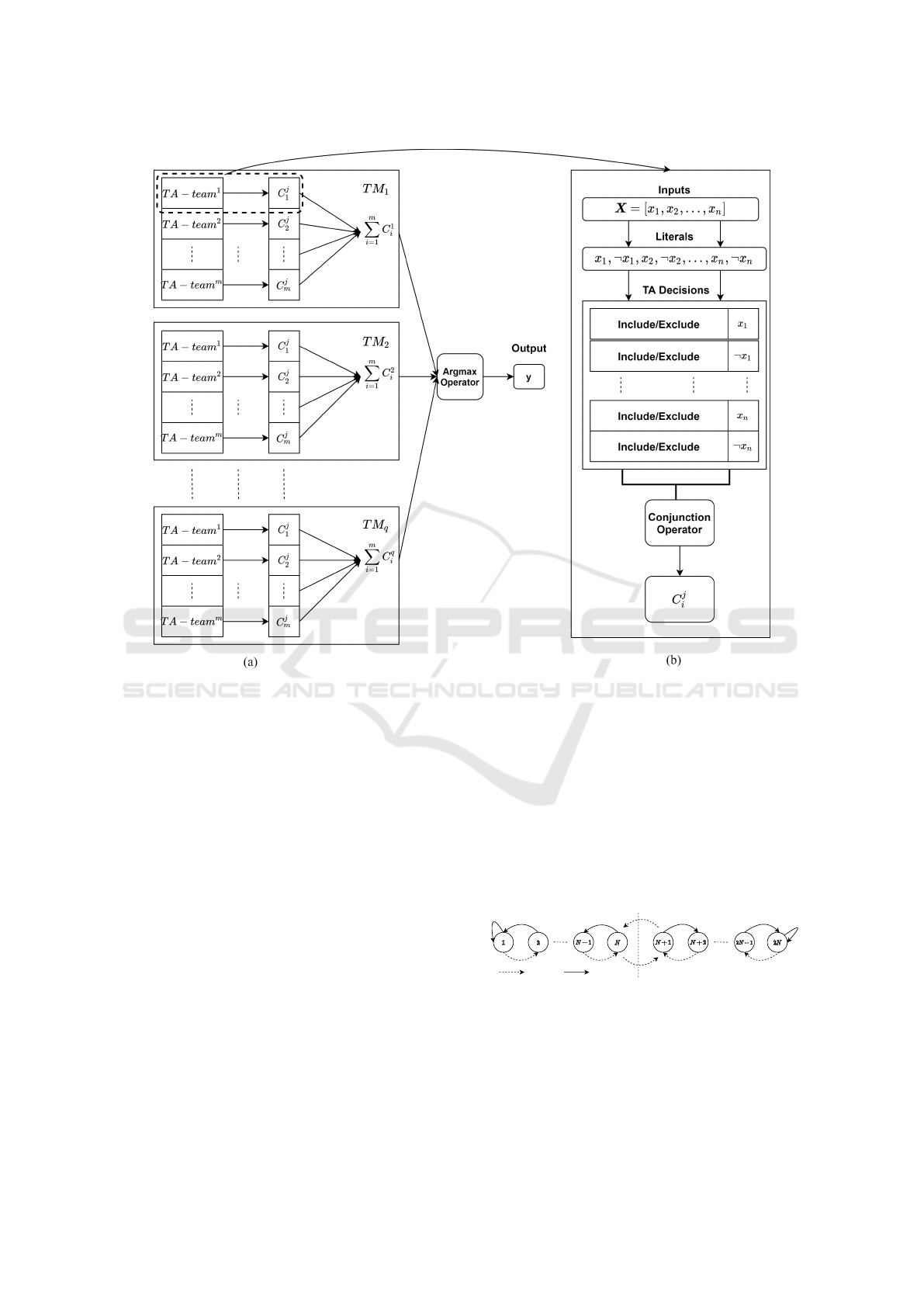
Figure 2: The architecture of (a) multiclass Tsetlin Machine, (b) a TA-team forms the clause C
j
i
, 1 ≤ j ≤ q, 1 ≤ i ≤ m.
In a multi-class TM, the final decision is made by
an argmax operator to classify the input based on the
highest sum of votes, as shown in Eq. (4):
y = argmax
j
f
j
(X)
. (4)
3.2 Training of the Proposed Scheme
The training of the TM is explained in detail in
(Granmo, 2018). Our focus here is how the word
senses are captured from data. Let us consider one
training example (X, ˆy). The input vector X – a bag
of words – represents the input to the TM. The target
ˆy is the sense of the target word.
Multiple teams of TAs are responsible for TM
learning. As shown in Fig. 2(b), a clause is assigned
one TA per literal. A TA is a deterministic automa-
ton that learns the optimal action among the set of ac-
tions provided by the environment. The environment,
in this particular application, is the training samples
together with the updating rule of the TA, which is
detailed in (Granmo, 2018). Each TA in the TM has
2N states and decides among two actions: Action 1
and Action 2, as shown in Fig. 3. The present state
of the TA decides its action. Action 1 is performed
from state 1 to N whereas Action 2 is performed for
states N + 1 to 2N. The selected action is rewarded or
penalized by the environment. When a TA receives a
reward, it emphasizes the action performed by mov-
ing away from the center (towards left or right end).
However, if penalty happens, the TA moves towards
the center to weaken the performed action, eventually
switching to the other action.
Action 1 Action 2
Penatly Reward
Figure 3: Representation of two actions of TA.
In TM, each TA chooses either to exclude (Action
1) or include (Action 2) its assigned literal. Based
on the decisions of the TA team, the structure of the
clause is determined and the clause can therefore gen-
erate an output for the given input X. Thereafter, the
state of each TA is updated based on its current state,
Interpretability in Word Sense Disambiguation using Tsetlin Machine
405

the output of the clause C
j
i
for the training input X ,
and the target ˆy.
We illustrate here the training process by way of
example, showing how a clause is built by exclud-
ing and including words. We consider the bag of
words for “Text Corpus 2”: (apple, like, orange, and
more) in Fig. 1, converted into binary form “Input
2”. As per Fig. 4, there are eight TAs with N = 100
states per action that co-produce a single clause. The
four TAs (TA to the left in Fig. 4) vote for the in-
tended sense with “more”, “like”, “orange”, and “ap-
ple”, whereas the four TAs (TA’ to the right in Fig. 4)
vote against it. The terms that are moving away from
the central states are receiving rewards, while those
moving towards the centre states are receiving penal-
ties. In Fig. 4, from the TAs to the left, we obtain
a clause
2
C
1
= “apple” ∧ “like”. The status of “or-
ange” is excluded for now. However, after observ-
ing more evidences from the “Input 2”, the TA of
“orange” is penalized for its current action, making
it change its action from exclude to include eventu-
ally. In this way, after more updates, the word “or-
ange” is to be included in the clause, thereby making
C
1
= “apple”∧“like”∧“orange”, increasing the preci-
sion of the sub-pattern and thereby the classification.
more
like
orange
more
like
Exclude Include IncludeExclude
1 2 100 101 102 200 1 2 100 101 102 200
TA TA'
apple
apple
orange
Figure 4: Eight TA with 100 states per action that learn
whether to exclude or include a specific word (or its nega-
tion) in a clause.
3.3 Interpretable Classification Process
We now detail the interpretability once the TM has
been trained. In brief, the interpretability is based on
the analysis of clauses. Let us consider the noun “ap-
ple” as the target word. For simplicity, we consider
two senses of “apple”, i.e., Company as sense s
1
and
Fruit as sense s
2
. The text corpus for s
1
is related to
the apple being a company, whereas for s
2
it is related
to the apple being a fruit.
Let us consider a test sample I
test
=
[apple, launch, iphone, next, year] and how its sense
is classified based on the context words. This set of
words is first converted to binary form based on a bag
of words as described earlier in Fig. 1.
2
As the clause describes a sub-pattern within the same
class, we ignore the superscript for different classes in no-
tation C
j
i
.
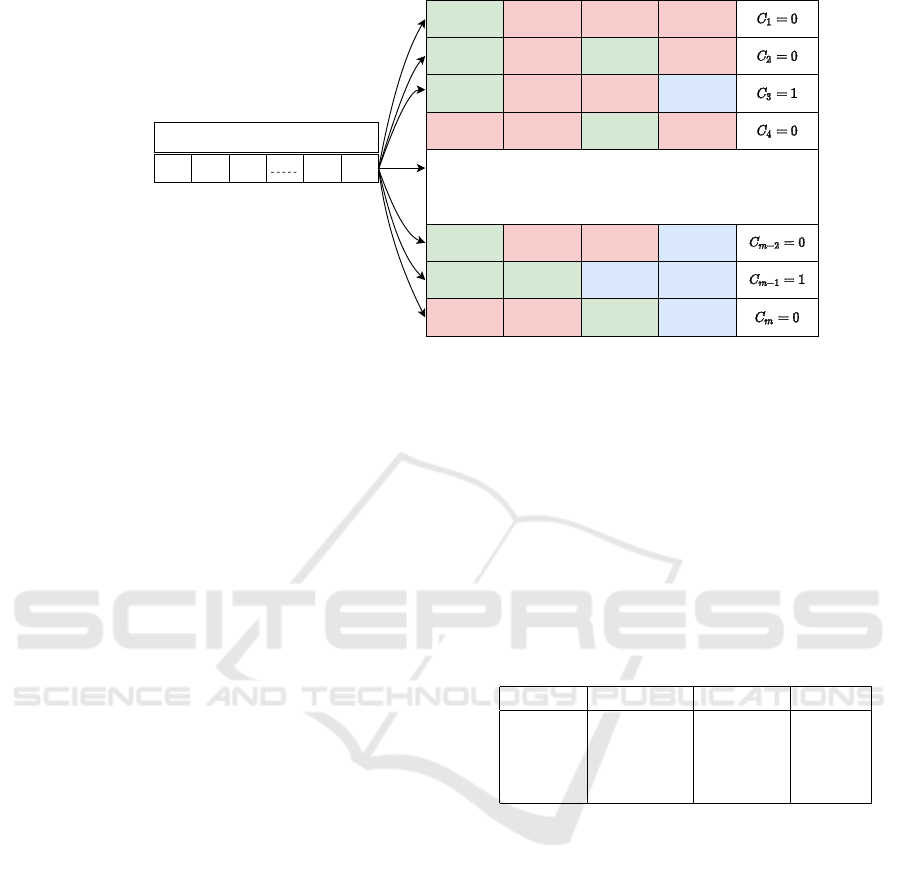
To extract the clauses that vote for sense s
1
, the
test sample I
test
is passed to the model and the clauses
that vote for the presence of sense s
1
are observed as
shown in Fig. 5. The literals formed by TM are ex-
pressed in indices of the tokens. For ease of under-
standing, it has been replaced by the corresponding
word tokens. The green box shows that the literal is
non-negated whereas the red box denotes the negated
form of the literal as shown in Fig. 5. For example, the
sub-patterns created by clause C
3
= apple∧¬orange∧
¬more. These clauses consist of included literals in
conjunctive normal form (CNF). Since the clauses in
the TM are trained sample-wise, there exist several
randomly placed literals in each clause. These ran-
dom literals just occur because of randomly picked
words that do not effect the classification. These lit-
erals are assigned to be non-important literals and
their frequency of occurrence is low. On the other
hand, the literals that has higher frequency among
the clauses are considered to be important literals
and hence makes significant impact on classification.
Here, we emphasize on separating important and non-
important literals for easy human interpretation. The
general concept for finding the important words for a
certain sense is to observe the frequency of appear-
ances for a certain word in the trained clauses. To do
that, in the above example, once the TM is trained,
the literals in clauses that output 1 or votes for the
presence of the class s
1
for I
test
are collected first, as
shown in Eq. (5):
L
t
=
[
k, j,
∀C
j
=1
{x
j
k
, ¬x
j
k
}, (5)
where x
j
k
is the k
th
literal, i.e., x
k
, that appears in
clause j and ¬x
j
k
is the negation of the literal. Note
that a certain literal x
k
may appear many times in L
t
due to the multiple clauses that output 1. Clearly, L
t
is
a set of literals (words) that appears in all clauses that
contribute to the classification of class s
1
. The next
step is to find frequently appearing literals (words) in
L
t
, which correspond to the important words. We de-
fine a function, β(h, H), which returns the number of
the elements h in the set H. We can then formulate
a set of the numbers for all literals x
k
and their nega-
tions ¬x
k
in L
t
, k ∈ {1, 2, . . . , n}, as shown in Eq. (6):
S
t
=
n
[
k=1:n
β(x
k
, L
t
),
[
k=1:n
β(¬x
k
, L
t
)
o
. (6)
We rank the number of elements in set S
t
in de-
scending order and consider the first η percent in the
rank as the important literals. Similarly, we define the
last η percent in the rank as non-important literals. To
distinguish the important literals more precisely, sev-
eral independent experiments can be carried out for a
ICAART 2021 - 13th International Conference on Agents and Artificial Intelligence
406
1 0 0 1 0
apple, launch, iphone, next, yearTokens
Binary input
0 1 2 k-1 kIndex
apple orange year NA
apple iphone NA NA
orange next year NA
orange like launch iphone
apple orange more NA
orange like apple more
apple like iphone orange
Figure 5: Structure of clauses formed by the combination of sub-patterns. Green color indicates the literals that are included
as original, red color indicates the literals that are included as the negated form and the blue color boxes indicates that there
are no literals because not all the clauses has same number of literals.
certain sense. Following the same concept, the literals
in M different experiments can be collected to one set
L
t
(total) as shown in Eq. (7):
L
t
(total) =
M
[
e=1
(L
t
)
e
, (7)
where (L
t
)
e
is the set of literals for the e
th
experi-
ment. Similarly, the counts of all literals in these ex-
periments, stored in set S
t
(total) shown in Eq. (8),
are again ranked and the top η percent is deemed as
important literals and the last η percent is the non-
important literals. The parameter η is to be tuned ac-
cording to the level of human interpretation required
for a certain task.
S
t
(total) =
(
[
k=1:n
β(x
k
, L
t
(total)),
[
k=1:n
β(¬x
k
, L
t
(total))
)
. (8)
4 EVALUATIONS
We present here the classification and interpretation
results on CoarseWSD-balanced dataset. There are
20 words having more than two senses to be classi-
fied. We select four of them to evaluate our model.
The reason for selecting only four words than using
all 20 words is that we want to show that TM pre-
serves interpretability with maintaining state-of-the-
art accuracy. So using only four words are enough
to represent the trade of between interpretability and
accuracy. The details of four datasets are shown in
Table 1. To train the TM for this task, we use the
same configuration of hyperparameters for all the tar-
get words. More specifically, we use the number of
clauses, specificity s and target T as 500, 5 and 80
for Apple and JAVA whereas 250, 3 and 30 for Spring
and Crane. After the model is trained for each target,
we validate our results using test data.
Table 1: Senses associated with each word that is to be clas-
sified.
Dataset Sense1 Sense2 Sense3
Apple fruit company NA
JAVA computer location NA
Spring hydrology season device
Crane machine bird NA
To illustrate the interpretability, let us take a sam-
ple as an example to extract the literals that are re-
sponsible for the classification of an input sentence:
“former apple ceo, steve jobs, holding a white
iphone 4”. Once this input is passed through the
model, TM predicts its sense as a company and we
examine the clauses that output 1. We append all the
literals that are presented in each clause and calculate
the number of appearances for each literal. The num-
ber of appearances of a certain literal for the selected
sample after one experiment is shown in Figs. 6 and 7
by a blue line. After five experiments, the number
for a certain literal is shown by a red line in Figs. 6
and 7. Clearly, it makes sense that the negated form
of the mostly-appearing literals in Fig. 6, i.e., “not
tree”, “not fruit”, “ not cherries” etc. indicate that the
word “apple” does not mean a fruit but a company.
Nevertheless, as stated in the previous section, there
are also some literals which are randomly placed in
Interpretability in Word Sense Disambiguation using Tsetlin Machine
407
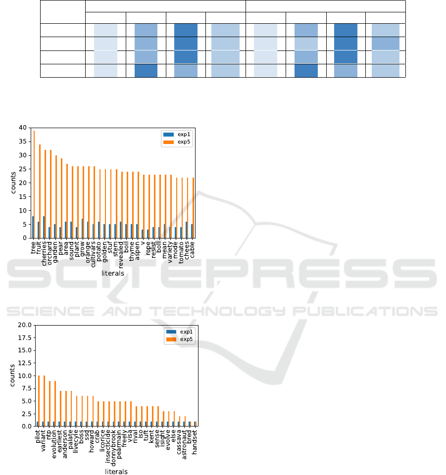
Table 2: Results on the full CoarseWSD balanced dataset for 4 different models: FastText-Base (FTX-B), FastText-
CommonCrawl (FTX-C), 1 Neural Network BERT-Base (BRT-B) and Tsetlin Machine (TM). Table cells are highlighted
(dark blue to light blue) for better visualization of accuracy.
Datasets
Micro-F1 Macro-F1
FTX-B FTX-C BRT-B TM FTX-B FTX-C BRT-B TM
Apple 96.3 97.8 99.0 97.58 96.6 97.7 99.0 97.45
JAVA 98.7 99.5 99.6 99.38 61.1 84.1 99.8 99.35
Spring 86.9 92.5 97.4 90.78 78.8 96.4 97.2 90.76
Crane 87.9 94.9 94.2 93.63 88.0 94.8 94.1 93.62
the clause and are non repetitive because the counts
refuse to climb up for the same input, marking them
not important literals, shown in Fig. 7.
Figure 6: Count of first 30 literals that are in negated form
for classifying the sense of apple as company. (considered
as important literals).
Figure 7: Count of last 30 literals that are in negated form
for classifying the sense of apple as company. (considered
as non-important literals.)
In addition to the interpretability of TM based ap-
proach, the accuracy is also an important parame-
ter for performance evaluation. Even though the se-
lected datasets have binary sense classification, we
will use Micro-F1 and Macro-F1 as the evaluation
metrics as shown in (Loureiro et al., 2020). Since,
interpretation of WSD is the main concern of the pa-
per, we will compare our work with the latest bench-
mark (Loureiro et al., 2020). Table 2 show the com-
parison of Macro and Micro F1 score on CoarseWSD
dataset for 4 different methods: FastText-Base (FTX-
B), FastText-CommonCrawl (FTX-C), 1 neural net-
work (NN) BERT base, and our proposed TM. FTX-
B is a fast text linear classifier without pre-trained
embeddings and FTX-C is a fast text linear classifier
with pre-trained embedding from Common Crawl.
These are considered as the standard baseline for
this dataset (Loureiro et al., 2020). Our proposed
TM based WSD easily outperforms FTX-B baseline
and is close to FTX-C without even considering the
pretrained embedding. However, TM falls short of
BERT’s performance given that it is a huge language
model that achieves the state-of-the-art performance
on most of the task. This shows that TM not only
possesses the interpretation of the WSD but also has
performance close to the state of the art.
5 CONCLUSIONS
This paper proposed a sense categorization ap-
proach based on recently introduced TM. Although
there are various methods for sense classification
on CoarseWSD-balanced dataset with good accuracy,
many machine learning algorithms fail to provide hu-
man interpretation that is used for explaining the pro-
cedure of particular classification. To overcome this
issue, we present a TM-based sense classifier that
learns the formulae form text corpus utilizing con-
junctive clauses to demonstrate a particular feature of
each category. Numerical results indicate that the TM
based approach is human-interpretable and it achieves
a competitive accuracy, which shows its potential for
further WSD studies. In conclusion, we believe that
the novel TM-based approach can have a significant
impact on sense identification that is a very important
factor in a chatbot or other WSD tasks.
ICAART 2021 - 13th International Conference on Agents and Artificial Intelligence
408

REFERENCES
Abeyrathna, K. D., Granmo, O.-C., Zhang, X., Jiao, L., and
Goodwin, M. (2019). The regression Tsetlin machine:
A novel approach to interpretable nonlinear regres-
sion. Philosophical Transactions of the Royal Society
A: Mathematical, Physical and Engineering Sciences,
378.
Agirre, E. and Edmonds, P. (2007). Word sense disambigua-
tion: Algorithms and applications. In Springer, Dor-
drecht.
Berge, G. T., Granmo, O., Tveit, T. O., Goodwin, M.,
Jiao, L., and Matheussen, B. V. (2019). Using the
Tsetlin machine to learn human-interpretable rules for
high-accuracy text categorization with medical appli-
cations. IEEE Access, 7:115134–115146.
Bhattarai, B., Granmo, O.-C., and Jiao, L. (2020). Mea-
suring the novelty of natural language text using the
conjunctive clauses of a Tsetlin machine text classi-
fier. ArXiv, abs/2011.08755.
Buhrmester, V., M
¨
unch, D., and Arens, M. (2019). Analysis
of explainers of black box deep neural networks for
computer vision: A survey.
de Lacalle, O. L. and Agirre, E. (2015). A methodology
for word sense disambiguation at 90% based on large-
scale crowdsourcing. In SEM@NAACL-HLT.
Devlin, J., Chang, M.-W., Lee, K., and Toutanova, K.
(2018). BERT: Pre-training of deep bidirectional
transformers for language understanding. arXiv
preprint arXiv:1810.04805.
Dongsuk, O., Kwon, S., Kim, K., and Ko, Y. (2018).
Word sense disambiguation based on word similarity
calculation using word vector representation from a
knowledge-based graph. In COLING.
Granmo, O.-C. (2018). The Tsetlin machine - a game theo-
retic bandit driven approach to optimal pattern recog-
nition with propositional logic.
Granmo, O.-C., Glimsdal, S., Jiao, L., Goodwin, M., Om-
lin, C. W., and Berge, G. T. (2019). The convolutional
Tsetlin machine.
Hadiwinoto, C., Ng, H. T., and Gan, W. C. (2019). Im-
proved word sense disambiguation using pre-trained
contextualized word representations.
K
˚
ageb
¨
ack, M. and Salomonsson, H. (2016). Word sense
disambiguation using a bidirectional LSTM. In Co-
gALex@COLING.
Khattak, F. K., Jeblee, S., Pou-Prom, C., Abdalla, M.,
Meaney, C., and Rudzicz, F. (2019). A survey of word
embeddings for clinical text. Journal of Biomedical
Informatics: X, 4:100057.
Lazreg, M. B., Goodwin, M., and Granmo, O.-C. (2020).
Combining a context aware neural network with a de-
noising autoencoder for measuring string similarities.
Computer Speech & Language, 60:101028.
Liao, K., Ye, D., and Xi, Y. (2010). Research on enter-
prise text knowledge classification based on knowl-
edge schema. In 2010 2nd IEEE International Confer-
ence on Information Management and Engineering,
pages 452–456.
Loureiro, D., Rezaee, K., Pilehvar, M. T., and Camacho-
Collados, J. (2020). Language models and word sense
disambiguation: An overview and analysis.
Mikolov, T., Sutskever, I., Chen, K., Corrado, G. S.,
and Dean, J. (2013). Distributed representations of
words and phrases and their compositionality. ArXiv,
abs/1310.4546.
Miller, G. A., Chodorow, M., Landes, S., Leacock, C., and
Thomas, R. G. (1994). Using a semantic concordance
for sense identification. In HLT.
Navigli, R., Camacho-Collados, J., and Raganato, A.
(2017). Word sense disambiguation: A unified evalu-
ation framework and empirical comparison. In EACL.
Navigli, R. and Velardi, P. (2004). Structural semantic in-
terconnection: A knowledge-based approach to word
sense disambiguation. In SENSEVAL@ACL.
Rezaeinia, S. M., Rahmani, R., Ghodsi, A., and Veisi, H.
(2019). Sentiment analysis based on improved pre-
trained word embeddings. Expert Systems with Appli-
cations, 117:139–147.
Rudin, C. (2018). Stop explaining black box machine learn-
ing models for high stakes decisions and use inter-
pretable models instead.
Sadi, M. F., Ansari, E., and Afsharchi, M. (2019). Super-
vised word sense disambiguation using new features
based on word embeddings. J. Intell. Fuzzy Syst.,
37:1467–1476.
Saha, R., Granmo, O.-C., and Goodwin, M. (2020). Mining
interpretable rules for sentiment and semantic relation
analysis using Tsetlin machines. In Artificial Intel-
ligence XXXVII, pages 67–78. Springer International
Publishing.
Sonkar, S., Waters, A. E., and Baraniuk, R. G.
(2020). Attention word embedding. arXiv preprint
arXiv:2006.00988.
Taghipour, K. and Ng, H. T. (2015). One million sense-
tagged instances for word sense disambiguation and
induction. In CoNLL.
Tripodi, R. and Pelillo, M. (2017). A game-theoretic ap-
proach to word sense disambiguation. Computational
Linguistics, 43(1):31–70.
Vaswani, A., Shazeer, N., Parmar, N., Uszkoreit, J., Jones,
L., Gomez, A. N., Kaiser, Ł., and Polosukhin, I.
(2017). Attention is all you need. In Advances in
neural information processing systems, pages 5998–
6008.
Wang, Y., Wang, L., Rastegar-Mojarad, M., Moon, S., Shen,
F., Afzal, N., Liu, S., Zeng, Y., Mehrabi, S., Sohn, S.,
and Liu, H. (2018). Clinical information extraction
applications: A literature review. Journal of Biomedi-
cal Informatics, 77:34 – 49.
Yadav, R. K., Jiao, L., Granmo, O.-C., and Goodwin,
M. (2021). Human-level interpretable learning for
aspect-based sentiment analysis. In The Thirty-Fifth
AAAI Conference on Artificial Intelligence (AAAI-21).
AAAI.
Yuan, D., Richardson, J., Doherty, R., Evans, C., and Al-
tendorf, E. (2016). Semi-supervised word sense dis-
ambiguation with neural models. In COLING.
Zhang, X., Jiao, L., Granmo, O.-C., and Goodwin, M.
(2020). On the convergence of Tsetlin machines
for the identity-and not operators. arXiv preprint
arXiv:2007.14268.
Zhong, Z. and Ng, H. T. (2010). It makes sense: A wide-
coverage word sense disambiguation system for free
text. In ACL.
Interpretability in Word Sense Disambiguation using Tsetlin Machine
409
