Detection of Malicious Binaries by Deep Learning Methods

Anantha Rao Chukka

and V. Susheela Devi

Defence Research and Development Organisation, India

Indian Institute of Science, Bengaluru, Karnataka, 560012, India

Keywords:

Malware Detection, Deep Learning Models, Convolutional Neural Networks, Malware Analysis, Portalble

Executable, Advanced Persistent Threats.

Abstract:

Modern day cyberattacks are complex in nature. These attacks have adverse effects like loss of privacy,

intellectual property and revenue on the victim institutions. These attacks have sophisticated payloads like

ransom-ware for money extortion, distributed denial of service(DDOS) malware for service disruptions and

advanced persistent threat(APT) malware to posses complete control over the victims computing resources.

These malware are metamorphic and polymorphic in nature and contains root-kit components to maintain

stealth and hide their malicious activity. So conventional defence mechanisms like rule-based and signature

based mechanisms fail to detect these malware. Modern approaches use behavioural analysis(static analysis,

dynamic analysis) to identity this kind of malware. However behavioural analysis process is hindered by

factors like execution environment detection, code obfuscation, anti virtualization, anti-debugging, analysis

environment detection etc. Behavioural analysis also requires domain expert to review the large amount of

logs produced by it to decide on the nature of the binary which is complex, time consuming and expensive.

To deal with these problems we proposed deep learning methods, where convolutional neural network model

is trained on the image representation of the binary to decide the binary nature as malicious or benign. In this

work we have encoded the binaries into images in a unique way. Deep convolution neural network is trained

on these images to learn the features to identify the binary as malicious or normal. The malware and benign

samples for the dataset creation are collected from online sources and windows operating system along with

compatible third party application software respectively.

1 INTRODUCTION

1.1 Malware Analysis

Malware(Mullins, 2017), short for malicious soft-

ware, consists of programming designed to disrupt or

deny operation,gather information that leads to loss of

privacy or exploitation, gain unauthorized access to

system resources, and other such abusive behaviour.

Some of the well known malware examples are tro-

jan, ransom-ware, boot-kit, root-kit etc. Analysing

malware provides deep insight into the activities per-

formed by the malware such as ﬁle-system modiﬁ-

cations, network connections established, persistent

and stealth activity and information gathering on the

victim’s computing resources. This information fa-

cilitates the security researchers to develop defence

mechanisms. Malware analysis is mainly categorized

into two types.

1. STATIC ANALYSIS (Ligh et al., 2010). In this

process the sample will be examined without run-

ning it, by specialized tools like dis-assemblers.

Static code analysis is the major component of

the static analysis which examines the instruc-

tion sequences to establish the execution be-

havioural characteristics. Meta information col-

lection is another component which collects ﬁle

meta-information like compiler environment, dig-

ital signatures, sample type and portable exe-

cutable ﬁle characteristics.

2. DYNAMIC ANALYSIS (Ligh et al., 2010). In this

process the sample activity will be monitored by

running it in contained environment. Various sys-

tem monitoring tools and techniques are used to

log the ﬁle-system, network, persistent and other

system activity.

132

Chukka, A. and Devi, V.

Detection of Malicious Binaries by Deep Learning Methods.

DOI: 10.5220/0010379701320139

In Proceedings of the 6th International Conference on Internet of Things, Big Data and Security (IoTBDS 2021), pages 132-139

ISBN: 978-989-758-504-3

1.2 Deep Learning

(Epelbaum, 2017) Deep learning methods are used

to learn data representations(features) at multiple ab-

straction levels by composing many layers of artiﬁ-

cial neural network units. The feature learning is hier-

archical where the starting layer represents low-level

features and the abstraction level increases with each

further layer. The major advantage of the deep learn-

ing methods is automatic learning of features by train-

ing on large amount of data without any human fea-

ture engineering. Our work uses convolutional neural

network, a kind of deep neural network speciﬁcally

used for computer vision applications.

1.2.1 Convolutional Neural Network (CNN)

(O’Shea and Nash, 2015), (Tutorial, 2017) The CNN

architecture consists of three major building blocks.

1. CONVOLUTIONAL LAYERS. These layers con-

sist of a number of ﬁlters. The convolution opera-

tion is expressed in terms of neural network oper-

ations where the ﬁlters represent the neurons. The

output of ﬁlter applied on previous layer is called

as a feature map.

2. POOLING LAYERS. These layers are used to

down sampling of the feature map. These lay-

ers are inserted after one or more convolutional

layers. The pooling layer reduces the over-ﬁtting

by generalizing the feature representations. It re-

duces the number of parameters in the following

layers leading to reduction in computation time.

3. FULLY CONNECTED LAYERS. These are gen-

eral feed forward neural network layers applied at

the end of convolution and pooling layers to com-

bine the features and make predictions of the net-

work.

The CNN also has operations like padding for proper

adjustment of ﬁlters at the image boundaries, normal-

ization for stable learning and regularization to reduce

the over-ﬁtting.

The Malware analysis procedures(Static analysis,

Dynamic analysis) have some disadvantages. Static

code analysis takes a long time and requires a do-

main expert to do the analysis. Code obfuscation

techniques hinder this process sometimes. Dynamic

analysis requires detection of the target execution en-

vironment which is complex. It also generates huge

logs and requires a domain expert to carry out the re-

view. Modern malware authors use techniques like

anti-debugging, anti-monitoring, virtual environment

detection, analysis environment detection which hin-

ders both the analysis techniques. Our approach is not

dependent on static and dynamic analysis. It directly

operates on raw binary thereby avoiding these difﬁ-

culties. The time required for deciding whether the

binary is malicious or not is minimal, once the deep

neural network training is completed.

The Malware detection process presented in this

paper has two major steps 1. Transforming the bi-

naries into images and 2. Training a deep convolu-

tional neural network on these images. The present

system design is focused on detecting 32-bit portable

executable binaries of Microsoft Windows Operat-

ing System. The Portable Executable (PE)(Goppit,

2006) format is a ﬁle format for executable, object

code, DLLs etc. used in 32-bit and 64-bit versions

of Windows operating systems. The proposed sys-

tem architecture is ﬁle format and operating system

independent. So the system can be easily extended to

other ﬁle formats and operating systems by training

the neural network on appropriate datasets.

The rest of this paper is organized as follows. Sec-

tion 2 describes the related work, Section 3 describes

the proposed malware detection system architecture ,

Section 4 describes results, Section 5 describes con-

clusion and Section 6 describes future work.

2 RELATED WORK

Recently machine learning methods especially deep

learning techniques are helping to solve some of

the complex problems in different problem domains.

Some authors used these techniques to detect mal-

ware and cluster malware into families. Joshua Saxe

and Konstantin Berlin (Saxe and Berlin, 2015) have

proposed a four layer deep feed-forward neural net-

work with feature vectors constructed by aggregation

of byte entropy, PE Imports and PE meta-data fea-

tures. Edward Raff et al.(Raff et al., 2017) have used

convolution neural networks with raw byte embed-

dings to detect the malware.

In earlier work we have used machine learning

models on feature sets like ﬁle meta information,

import functions, opcode sequences, API sequences,

API Normal and custom ﬂags to classify the binary

as malware or benign. We created different meta

datasets by combining the predictions of multiple ma-

chine learning models on individual feature sets to im-

prove the classiﬁcation accuracy. This system is de-

pendent on static and dynamic malware analysis. So

it encounters the same problems like execution envi-

ronment detection, anti-debugging etc. as discussed

in Section 1.

Lakshmanan Nataraj et al.(Nataraj et al., 2011)

have used visualization and automatic classiﬁcation

Detection of Malicious Binaries by Deep Learning Methods

133

Figure 1: System Architecture.

of malware into families by treating malware binaries

as grey scale images where raw bits represent pixels.

They extracted GIST features(Torralba et al., 2003)

from these images and used k-NN classiﬁer to classify

them. Our approach also uses similar thought process

by treating binaries as images. However our system

differs in following ways

1. IMAGE CREATION. Our image constructing pro-

cess completely differs from Lakshmanan Nataraj

et al.(Nataraj et al., 2011). We transformed bi-

naries into colour images by treating opcodes as

colour coded pixels instead of treating raw bits as

grey scale pixels. This approach has advantages in

capturing the patterns in malware instruction se-

quences. The raw byte grey scale image is noisy

because PE binary has lot of sections which varies

frequently and have little impact on behavioural

patterns of the binary.

2. LEARNING PROCESS. We used deep learning

techniques to learn the features automatically and

predict the unknown binary category instead of

the traditional k-NN classiﬁer over GIST features.

3 PROPOSED SYSTEM

The proposed system architecture is depicted in Fig-

ure 1. In the ﬁrst stage datasets are created by trans-

forming the binaries(both benign and malware) into

colour images by mapping the opcodes in the binary

to colour pixels. Next a deep convolutional neural net-

work is trained on the image datasets to learn the fea-

ture ﬁlters and weights of the network. Later these

parameters( feature ﬁlters + weights) are used to pre-

dict the unknown binary as malware or benign.

3.1 Sample Collection

Deep learning models are dependent on large amount

of quality data to learn better feature representa-

tions. The information security researchers world-

wide are maintaining the repositories of malware for

the collaborative research and developing defence

mechanisms. Lenny Zeltser(Zeltser, 2020) com-

piled some of the well known resources which in-

cludes Contagio malware dump(MilaParkour, 2020),

VirusShare(Mellissa, 2020) and Malwr(Community,

2017) repository. We have collected 12500 malware

samples from the VirusShare(Mellissa, 2020) for the

present experiment.

Benign Portable Executable(PE) ﬁles are col-

lected by ﬁltering application/x-msdownload(MSDN,

2016) Multi-purpose Internet Mail Extension(MIME)

from Operating System and third party application

software ﬁles. The ﬁles have 5MB size restriction.

Total 12500 benign PE ﬁles are used for the current

experiment. The major reason behind the size restric-

tion is to avoid large software ﬁles which are gener-

ally used as carriers for the smaller size malware pay-

loads. The large ﬁles also generate millions of op-

codes which makes the image creation process time

consuming and computationally expensive. All the

samples(both malware and normal) are windows 32-

bit architecture compatible. Windows 32-bit and 64-

bit executables differ in the instruction types, align-

ments and other architectural characteristics. So mix-

ing both types of executables will lead to noisy and

inaccurate data.

3.2 Image Creation

The image creation has following three major steps

and Algorithm 1 describes the image creation process

in detail.

1. Collect unique opcodes over the complete sample

collection.

2. Map each opcode to unique colour code.

3. Transform each sample into image by arranging

the opcodes in given image shape and replacing

opcodes with respective colour codes.

3.3 Datasets

We have created two types of datasets from the sam-

ple collection.

1. TYPE1. It is a dataset with 384 × 384 size three

channel colour images created by arranging op-

codes into 384 ×384 grid and mapping them with

respective colour codes.

2. TYPE2. It is a dataset with 384 × 384 size three

channel colour images created using 8 × 8 sub-

grids of opcodes. The sub-grids are used to ex-

ploit the spatial correlation among the instruction

sequences. The opcodes in sub-grids are mapped

to respective colour codes to form the image.

We have used a total of 25000(12500 Normal + 12500

Malicious) samples for the dataset creation. The par-

IoTBDS 2021 - 6th International Conference on Internet of Things, Big Data and Security

134

Algorithm 1: Sample Binary to Image Conversion.

1: procedure CONVERTTOIMAGES(source, destination,

size)

2: for all sample ∈ source do

3: opcodes ← ExtractOpCodes(sample) . ∗1

4: SaveToFile(opcodes, destination)

5: end for

6: opcode set ← Φ

7: for all sample ops ∈ destination do

8: opcode set ← opcode set ∪ sample ops . ∗2

9: end for

10: color mapper ← {}

11: for all opcode ∈ opcode set do

12: color code ← GetRGBCode() . ∗3

13: color mapper[opcode] ← color code

14: end for

15: color mapper[pad code] ← pad color

16: for all sample ops ∈ destination do

17: t grid ← CGrid(size, sample ops) . ∗4

18: s img ← mapper(t grid, color mapper)

19: SaveToFile(s img, destination)

20: end for

21: end procedure

• ∗1: ExtractOpcodes uses python diStorm (Dabah,

2020) library to collect opcodes

• ∗2: Union Collects Unique Opcodes

• ∗3: GetRGBCode returns unique color code which is

not present in color mapper

• ∗4: CGrid returns opcodes arranged in grid with given

size(width, height). If opcodes exceeds the size it dis-

cards remaining opcodes. Otherwise it pads the grid

with default padding code

titioning of the dataset into train, validations and test

set is as follows.

• TRAINING. 18000 Samples (9000 from each

class i.e Normal and Malicious)

• VALIDATION. 2000 Samples (1000 from each

class i.e Normal and Malicious)

• TEST. 5000 Samples (2500 from each class i.e

Normal and Malicious)

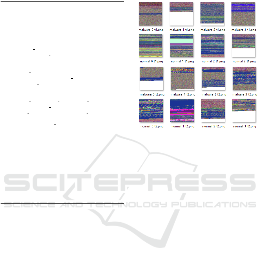
Figure 2 provides some of the example sample images

of the datasets.

3.4 Convolution Neural Network

(Howard and Thomas, 2020), (Chollet, 2020) and

(Team, 2020) The Convolutional neural network ar-

chitecture is depicted in Figure 3. The model has 6

convolution layers, 3 Max-pooling layers along with

fully connected network of 2 dense layers and one bi-

nary output layer.

Each convolution layer is equipped with 10 per-

cent dropout to reduce over-ﬁtting and batch normal-

ization for stable learning. The convolution layers

• malware ∗ t[1|2]: Type[1|2] Malware Images

• normal ∗ t[1|2]: Type[1|2] Normal Images

Figure 2: Example Samples.

uses zero-padding to make the ﬁlters ﬁt properly at

the image borders. 2 × 2 size Max-pooling is applied

after every two convolutions with stride 2 on both di-

mensions. All convolution layers are used RELU acti-

vation units. 3 ×3 size convolution ﬁlters are doubled

for every two convolution layers.

The dense layers are equipped with 50 percent

drop out on each layer to reduce over-ﬁtting. The

batch normalization is applied on each layer for sta-

ble learning. The dense layers have 256 units on each

layer with RELU activation units. The binary output

layer uses SIGMOID activation unit which is most suit-

able for binary classiﬁcation.

Since our problem is in binary classiﬁcation do-

main, we have compiled the model with the following

parameters.

• RMSPROP. Optimizer

• BINARY CROSS-ENTROPY. Loss function

• ACCURACY. is performance metric.

3.5 Training

(Howard and Thomas, 2020), (Chollet, 2020) and

(Team, 2020) We have used model ensemble for bet-

ter performance. Four models are trained on the data.

Each model training is described as follows along

with hyper parameters.

• BATCH SIZE. The batch size is ﬁxed at 16.

Detection of Malicious Binaries by Deep Learning Methods

135

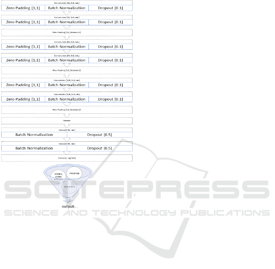
Figure 3: Model Architecture.

• EPOCHS. 50 epochs are used in total.

• LEARNING RATE. Dynamic learning rate is

used. The ﬁrst epoch is trained with learning rate

0.001. The next 4 epochs used 0.1, after that 15

epochs used 0.01 and later 30 epochs used 0.001.

Data augmentation is used on training data to improve

the performance. Two types of models are saved.

1. Best Accuracy Model. A model with best accu-

racy(maximum accuracy) over 50 epochs.

2. Least Loss Model. A model with minimum

loss(minimum loss) over 50 epochs

The ﬁnal models are constructed as follows

• MEAN CLASSIFIER(ACCURACY). Average ac-

curacy over four best accuracy models.

• MEAN CLASSIFIER(LOSS). Average accuracy

over four least loss models

The training is performed on NVIDIA Tesla K40c

with 12GB GPU memory. The development envi-

ronment is in Python with Kearas API with Tensor-

Flow backend. The training time per epoch is approx-

imately 18 minutes. The total training time per dataset

is 60hours ( 15H per model * 4 Models).

3.6 Challenges Faced

we have faced the following challenges during the de-

velopment.

• Batch Size. We are unable to perform the training

with large batch sizes because of the GPU mem-

ory restriction. The batch size is restricted to 16.

• Image Size. The average opcodes per binary is

206485. However we restricted the image size to

384 × 384 = 147456 pixels. The reason behind

this is that convolution takes longer time with in-

creasing image size.

• Hyper Parameter Tuning. We are able to ex-

periment with small number of values for hyper

parameters like DROPOUT, NUMBER OF CONVO-

LUTION LAYERS, POOLING SIZE AND FILTERS

PER LAYER because of the longer training time

and hardware constraints.

• Diversity of Binaries. Normal binaries are col-

lected from the operating system and limited third

party software. So the samples may not be di-

verse as real time normal ﬁles. At the same

time we have not established the diversity in the

VirusShare samples which we have used for our

malware category.

All these challenges will be addressed in future work.

4 RESULTS

4.1 Type1 Dataset

Figure 4 shows that the training of models with Type1

dataset is smooth over the 50 epochs. Some ﬂuctua-

tion is there with validation loss. However mostly it

progressed towards minimum direction except for the

MODEL0 which is random over the 50 epochs period.

It shows that the MODEL0 is struggling to ﬁnd its op-

timum weights. This behaviour of MODEL0 is cor-

roborated with the accuracy curves in Figure 6 where

MODEL0 validation accuracy is not in agreement with

the training accuracy for most of the time. All re-

maining model accuracies are in agreement with the

training accuracy in large part of the training phase.

This clearly indicates the models are not over-ﬁtting

the data.

The ensemble of the models is used when the

model performance is poor. In this case MODEL0

IoTBDS 2021 - 6th International Conference on Internet of Things, Big Data and Security

136

Table 1: Classiﬁcation accuracy with best accuracy model.

CLASSIFIER

DATA MODEL0 MODEL1 MODEL2 MODEL3 MEAN

SET VALID TEST VALID TEST VALID TEST VALID TEST VALID TEST

ACC 0.9710 0.9724 0.9765 0.9792 0.9740 0.9748 0.9805 0.9796 0.9755 0.9765

TYPE1 LOSS 0.1333 0.1291 0.0990 0.0808 0.1286 0.1259 0.0834 0.0855 0.1110 0.1053

ACC 0.9835 0.9776 0.9805 0.9758 0.9815 0.9710 0.9785 0.9750 0.9810 0.9748

TYPE2 LOSS 0.0759 0.0954 0.1731 0.1753 0.1142 0.1244 0.1174 0.1369 0.1202 0.1330

Table 2: Classiﬁcation accuracy with least loss model.

CLASSIFIER

DATA MODEL0 MODEL1 MODEL2 MODEL3 MEAN

SET VALID TEST VALID TEST VALID TEST VALID TEST VALID TEST

ACC 0.9670 0.9681 0.9760 0.9748 0.9645 0.9692 0.9785 0.9780 0.9715 0.9725

TYPE1 LOSS 0.1013 0.0960 0.0949 0.0950 0.1167 0.1102 0.0832 0.0810 0.0990 0.0955

ACC 0.9835 0.9776 0.9760 0.9738 0.9795 0.9754 0.9765 0.9742 0.9789 0.9752

TYPE2 LOSS 0.0759 0.0954 0.0938 0.0970 0.0848 0.0917 0.1006 0.1087 0.0888 0.0982

performance is poor. We take average of the perfor-

mance of four models results to give our ﬁnal predic-

tion. Due to this the prediction will be robust and the

ensemble also helps in improving the classiﬁer per-

formance.

By averaging the results of multiple models, the

performance of our model prediction is robust and

also improves the performance of our ﬁnal prediction.

Tables 1 and 2 provide the accuracy and loss with re-

spect to different models compared with model en-

semble(Mean) model. Type1 dataset achieved 97.65

percent accuracy with Mean model(Accuracy) and

97.25 percent with Mean model(Loss). There is

a small difference between the validation and test

datasets losses and validation and test datasets accu-

racies per model, and is consistent across all models.

It clearly indicates that the model prediction is con-

sistent with increasing unknown data(Validation and

Test datasets sizes are 2000 and 5000 respectively).

We can conclude from this result along with the accu-

racy comparison with training data from Figure 6 that

the model is generalized properly without over-ﬁtting

on the training data.

4.2 Type2 Dataset

The training with Type2 dataset is not smooth as it

was in Type1 dataset. This can be observed from

Figures 7 and 8. The validation loss curves are ran-

domly ﬂuctuating. From Figure 9 we can observe that

the validation accuracy is slightly deviating from the

training accuracy over a lot of epochs. This clearly

indicates that the model is over-ﬁtting the data. This

can be observed from the results provided in Tables

1 and 2. The Mean model(accuracy) has 98.10 per-

cent accuracy with validation data and 97.48 percent

accuracy with test dataset. In the same manner Mean

model(Loss) has 97.89 percent accuracy with valida-

tion data and 97.52 percent of accuracy with test data.

This clearly shows that the model performance is de-

teriorating fast as unknown data increases as com-

pared to Type1 dataset.

Even though Type2 dataset is unable to generalize

well compared to Type1 dataset, it has the following

advantages

• The validation accuracy of Type2 dataset from

both(accuracy, loss) Mean models is more com-

pared to Type1 dataset. So with proper tuning

of regularization parameters we can achieve good

performance by reducing the over-ﬁtting.

• The Type2 dataset over-ﬁtting margin is large

compared to Type1 dataset. However it is still

a reasonable model because the margin is small

(around 0.5 percent accuracy difference).

Our deep learning model has achieved 97.65% accu-

racy with training on 18000 samples which is better

than the Edward Raff et al.(Raff et al., 2017) approach

in their work titled ’Malware Detection by Eating a

Whole EXE’ where they achieved 94% accuracy with

training on 2 million corpus.

Detection of Malicious Binaries by Deep Learning Methods

137

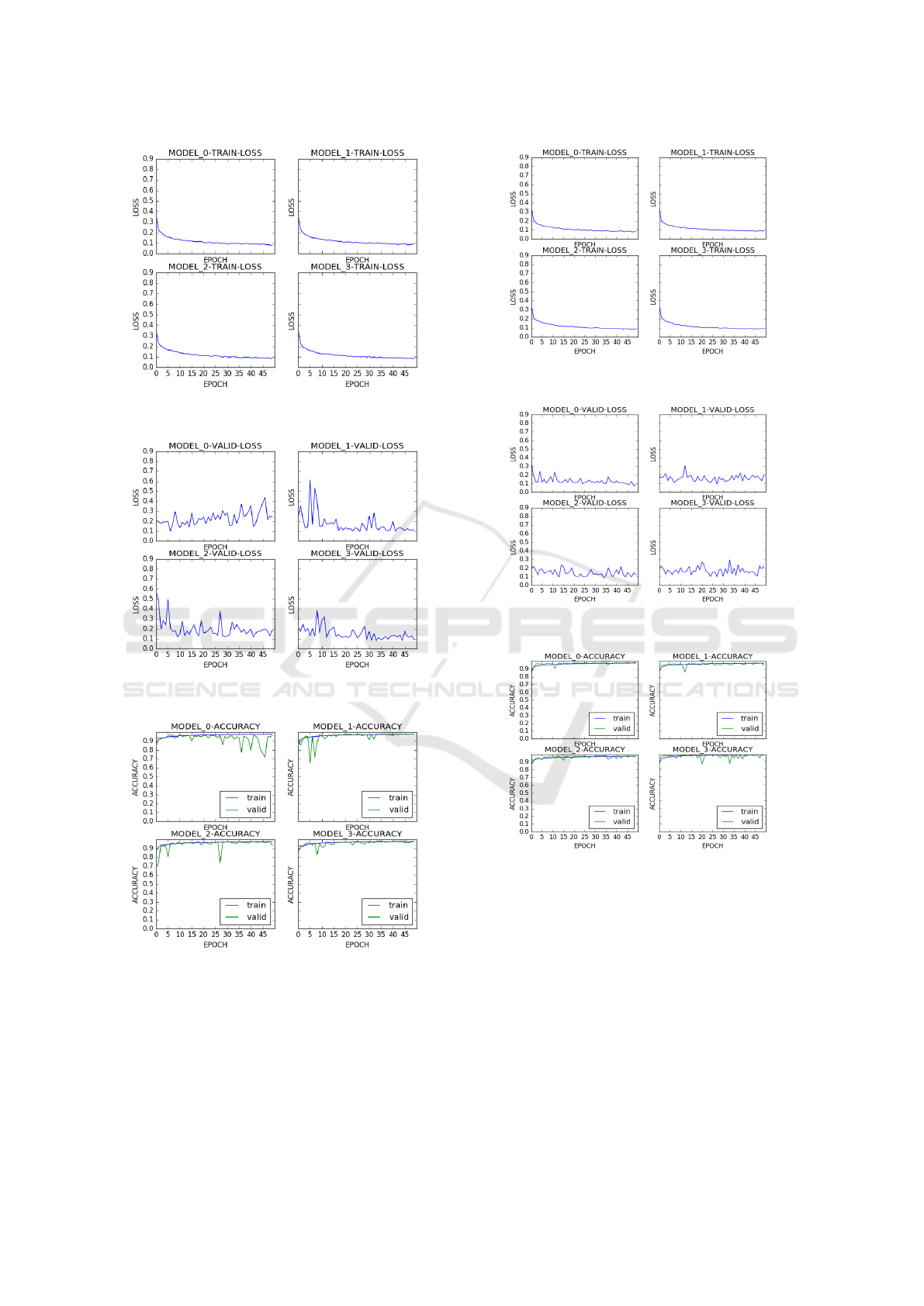
Figure 4: Type1 Dataset Training Loss.

Figure 5: Type1 Dataset Validation Loss.

Figure 6: Type1 Dataset Accuracy.

5 CONCLUSION

In this paper we have presented detection of malicious

windows binaries with deep learning approaches. The

windows binaries are converted into colour images

by extracting opcodes from the binaries and map-

Figure 7: Type2 Dataset Training Loss.

Figure 8: Type2 Dataset Validation Loss.

Figure 9: Type2 Dataset Accuracy.

ping them into colour pixels. Convolutional neural

network is trained on these images to learn the fea-

tures ﬁlters and weights of the network. Two types

of datasets are used for training, Type1 dataset is

383 × 384 pixel images where each image is created

by arranging the opcodes in 383 × 384 grid and map-

ping them into respective colour codes, Type2 dataset

also has 383 × 384 pixel images where each image

is created by arranging opcodes blocks of size 8 × 8

and mapping opcodes in block into respective colour

codes. Two types of models (Best accuracy, Least

Loss) are saved for the prediction. Model ensem-

IoTBDS 2021 - 6th International Conference on Internet of Things, Big Data and Security

138

ble is used where multiple models are trained on the

dataset and the ﬁnal models(Mean accuracy, Mean

Loss) are constructed by taking the average of the

results. The results show that Type1 dataset learn-

ing is smooth and produced 97.65% accuracy with

Mean accuracy model and 97.25% with Mean loss

model. Type2 dataset is somewhat over-ﬁtting the

data and produced 97.48% accuracy with Mean ac-

curacy model and 95.52% accuracy with mean loss

model. However Type2 dataset performance can be

improved by adjusting the regularization parameters

because it has high validation accuracy. In this work

we have used deep learning methods on the image

representations of the binaries to detect the nature of

the binary as malicious or benign. This mechanism is

unique in nature by working directly on raw binaries

thus avoiding all the difﬁculties in malware analysis

process. The accuracy of our model is more than 97

percent which is reasonably good in the malware de-

tection domain.

6 FUTURE WORK

We plan to experiment with the models by tuning

the parameters of the network to improve the accu-

racy. We are also planning to extend this mecha-

nism to other ﬁle formats like Microsoft Ofﬁce doc-

uments(Word, Power Point, Excel), Portable Doc-

ument Format(PDF) and Web Application(HTML,

HTA, JS) and Operating Systems like Linux, MacOS

by training the model on appropriate ﬁle formats.The

current mechanism assigns unique colour codes to

unique opcodes. However we are trying to assign

colour code mapping per group basis where opcodes

are placed in groups based on their functional simi-

larities like data transfer, control instructions etc. The

future work will also address the challenges described

in Section 3.

REFERENCES

Chollet, F. (2020). Keras: The Python Deep Learn-

ing library - The Sequential model. https://keras.io/

getting-started/sequential-model-guide/.

Community, C. S. (2017). Malwr (Free malware analysis

service). https://malwr.com/.

Dabah, G. (2020). Powerful Disassembler Library For

x86/AMD64. https://github.com/gdabah/distorm.

Epelbaum, T. (2017). Deep learning: Technical introduc-

tion. arXiv:1709.01412. https://arxiv.org/pdf/1709.

01412.pdf.

Goppit (2006). Portable executable ﬁle format – a re-

verse engineer view. CodeBreakers Magazine (Se-

curity & Anti-Security- Attack & Defense), 1 issue

2. http://index-of.es/Windows/pe/CBM 1 2 2006

Goppit PE Format Reverse Engineer View.pdf.

Howard, J. and Thomas, R. (2020). Practical Deep Learn-

ing For Coders. http://course.fast.ai/.

Ligh, M., Adair, S., Hartstein, B., and Richard, M. (2010).

Malware Analyst’s Cookbook and DVD: Tools and

Techniques for Fighting Malicious Code. Wiley Pub-

lishing.

Mellissa (2020). VirusShare (Repository of malware sam-

ples). https://virusshare.com/.

MilaParkour (2020). Contagio (Malware Dump). http://

contagiodump.blogspot.com/.

MSDN (2016). MIME Type Detection in Windows Internet

Explorer. https://msdn.microsoft.com/en-us/library/

ms775147(v=vs.85).aspx.

Mullins, D. P. (2017). Introduction to Computing, chapter

5.4. Online.

Nataraj, L., Karthikeyan, S., Jacob, G., and Manjunath,

B. S. (2011). Malware images: Visualization and au-

tomatic classiﬁcation. International Symposium on Vi-

sualization for Cyber Security(VizSec’11).

O’Shea, K. and Nash, R. (2015). An introduction to convo-

lutional neural networks. ArXiv e-prints.

Raff, E., Barker, J., Sylvester, J., Brandon, R., Catanzaro,

B., and Nicholas, C. (2017). Malware detection by

eating a whole exe. arXiv:1710.09435v1.

Saxe, J. and Berlin, K. (2015). Deep neural network based

malware detection using two dimensional binary pro-

gram features. arXiv:1508.03096v2.

Team, G. B. (2020). An open-source software library for

Machine Intelligence. https://www.tensorﬂow.org/.

Torralba, A., Murphy, K. P., Freeman, W. T., and Rubin,

M. A. (2003). Context-based vision system for place

and object recognition. International Conference on

Computer Vision.

Tutorial, S. U. (2017). Convolutional Neural Net-

work. http://uﬂdl.stanford.edu/tutorial/supervised/

ConvolutionalNeuralNetwork/.

Zeltser, L. (2020). Malware Sample Sources

for Researchers. https://zeltser.com/

malware-sample-sources/.

Detection of Malicious Binaries by Deep Learning Methods

139