Detection of Malicious Binaries by Applying Machine Learning Models

on Static and Dynamic Artefacts

Anantha Rao Chukka

and V. Susheela Devi

Defence Research and Development Organisation, India

Indian Institute of Science, Bengaluru, Karnataka, 560012, India

Keywords:

Malware Detection, Machine Learning Models, Malware Analysis, API Sequences, Opcode Sequences,

Import Function, File Meta Information, Malware Operational Patterns, Portable Executable, Artiﬁcial Neural

Network, Support Vector Machine, Random Forest, Naive Bayes, K-nearest Neighbour.

Abstract:

In recent times malware attacks on government and private organizations are rising. These attacks are carried

out to steal conﬁdential information which leads to loss of privacy, intellectual property issues and loss of

revenue. These attacks are sophisticated and described as Advanced Persistent Threats(APT). The payloads

used in this type of attacks are polymorphic and metamorphic in nature and contains stealth and root-kit

components. As a result the conventional defence mechanisms like rule-based and signature-based methods

fail to detect these malware. So modern approaches rely on static and dynamic analysis to detect sophisticated

malware. However this process generates huge log ﬁles. The domain expert needs to review these logs to

classify whether the binary is malicious or benign which is tedious, time consuming and expensive. Our

work uses machine learning models trained on the datasets, created using the analysis logs, to overcome these

problems. In this paper a number of supervised machine learning models are presented to classify the binary

as malicious or benign. In this work we have used automated malware analysis framework to collect run time

behavioural artefacts. Static analysis mainly focuses on collecting binary meta information, import functions

and opcode sequences. The dataset is created by collecting malware from online sources and benign ﬁles from

windows operating system and third party software.

1 INTRODUCTION

Malware(Mullins, 2017), short for malicious soft-

ware, consists of programming designed to disrupt or

deny operation,gather information that leads to loss

of privacy or exploitation, gain unauthorized access

to system resources, and other abusive behaviour. Ex-

amples of malware include virus, worm, trojan, spy-

ware, ad-ware, root-kit and boot-kit etc. Malware

analysis detects and develops defence mechanisms

against the malware attacks by exploring various ac-

tivities of malicious software like its payload, persis-

tence mechanism and stealth features. The analysis is

categorized in two ways, static analysis and dynamic

analysis.

1. STATIC ANALYSIS (Michael Ligh and Richard,

2010). In this process the artefacts are collected

without running the binary. This process includes

static code analysis by disassembling the binary,

collection of meta information like author, digital

signatures, ﬁle hashes, creation dates, portable ex-

ecutable(PE) characteristics and strings present in

the binary.

2. DYNAMIC ANALYSIS (Michael Ligh and

Richard, 2010). In this process the run time

behavioural artefacts are collected by executing

the binary in contained environment. This process

collects information like ﬁle-system, process,

network and registry activity etc.

The Malware detection process presented in this pa-

per has two major steps 1. Performing static and dy-

namic analysis. and 2. Applying machine intelligence

on analysis logs to classify the binary.

The proposed system is intended for detecting

Portable Executable malware targeting Microsoft

Windows Operating System. The Portable Executable

(PE)(Goppit, 2006) format is a ﬁle format for exe-

cutables, object code, DLLs etc. used in 32-bit and

64-bit versions of Windows operating systems. The

main reason for this is that, at present the automated

malware analysis framework is currently available for

Microsoft Windows only. The proposed system can

Chukka, A. and Devi, V.

Detection of Malicious Binaries by Applying Machine Learning Models on Static and Dynamic Artefacts.

DOI: 10.5220/0010379600290037

In Proceedings of the 6th International Conference on Internet of Things, Big Data and Security (IoTBDS 2021), pages 29-37

ISBN: 978-989-758-504-3

be extended in future for other platforms like Linux

and Mac-OS by developing corresponding analysis

engines.

The rest of this paper is organized as follows. Sec-

tion 2 describes the related work, Section 3 describes

the proposed malware detection system architecture ,

Section 4 describes results, Section 5 describes con-

clusion and Section 6 describes future work.

2 RELATED WORK

Several behavioural analysis tools have been devel-

oped over the past decade to detect sophisticated mal-

ware. Some of the tools are proprietary in nature

and some are open-source. Cuckoo malware anal-

ysis(Team, 2020a) is one of the well known open

source frameworks of this kind. Buster Sandbox An-

alyzer((BusterBSA), 2020) is another freeware tool

that has been designed to analyze the behaviour of

processes and the changes made to system and then

evaluate if they are malware suspicious. ThreatAn-

alyzer(Vipre(ThreatTrack), 2020) is one of the com-

mercially available software to perform automatic

malware analysis. Some authors applied machine

learning techniques on the logs generated by these

tools to infer whether the sample is malicious or not.

Some authors clustered the malware samples to iden-

tify malware families. Approaches used are discussed

below.

Smita Ranveer and Swapnaja Hiray(Ranveer and

Hiray, 2015) discussed SVM classiﬁer on opcode

sequences and API(Application Programming Inter-

face) sequences from behavioural analysis as fea-

tures to identify the nature of the sample. Konrad

Rieck et al.(Rieck et al., 2011) proposed a new en-

coding mechanism of the dynamic behavioural logs

from CWSSandbox(Vipre(ThreatTrack), 2020). They

called it as MIST(Malware Instruction Set) as it re-

sembles the general processor instruction set formats.

They formed Q-gram sequences on the MIST to em-

bed the malware report as a vector of large dimen-

sion with binary numbers. They used clustering algo-

rithms on these vectors to identify the malware fami-

lies. P. V. Shijo and A. Salim(Shijo and Salim, 2015)

used strings and API sequences as the feature set and

applied SVM and random forest models to classify

the samples. Igor Santos et al.(Santos et al., 2013)

used opcode mutual information gain as feature selec-

tion for static malware analysis and indicator features

of monitored actions in dynamic analysis to perform

the classiﬁcation.

We use four additional feature sets, 1. Im-

port Functions, 2. Application Programming Inter-

face(API) calls generally exploited by malware au-

thors, 3. Custom ﬂags which represent the malware

operational patterns and 4. Portable Executable(PE)

ﬁle format characteristics along with opcode se-

quences and API sequences to improve the classiﬁ-

cation accuracy.We also use multi level classiﬁcation

along with classiﬁer stacking to improve the classi-

ﬁcation accuracy. Our dataset creation procedure is

unique where features of same kind are grouped to-

gether to make a feature set. This process has the fol-

lowing advantages

• Weighting of features based on their importance

impacts the classiﬁer performance. However tun-

ing of these parameters is computationally expen-

sive with more number of features. This problem

can be solved by weighting the feature sets rather

than individual features.

• Users have ﬂexibility to build various derived

datasets based on their requirement from these

feature sets.

• Dimensionality reduction can be applied at fea-

ture set level rather than entire dataset level.

3 PROPOSED SYSTEM

The proposed system architecture is depicted in

Figure 1. The Automated malware analysis en-

gine, based on API hooking technology(Michael Ligh

and Richard, 2010) ((BusterBSA), 2020)(Hunt and

Brubacher, 1999) is used to collect dynamic be-

haviour artefacts of the binary. Samples are exe-

cuted in controlled environment created using Vir-

tualisation Software. The guest system is equipped

with Windows 7 Operating System. Static anal-

ysis artefacts are collected using python PE utili-

ties(Carrera, 2020)(Tek, 2020) and diStorm3(Dabah,

2020) library. Three types of derived datasets are cre-

ated from the original dataset by multiple classiﬁer

predictions, trained on individual feature sets of the

original dataset. The classiﬁcation accuracy is im-

proved with derived datasets compared to the indi-

vidual feature sets. So the ﬁnal classiﬁcation of the

sample whether it is malware or benign is obtained

using derived datasets.

3.1 Sample Collection

Machine learning models are driven by the data,

so sample collection by quality and quantity is an

important process. Security researchers worldwide

are maintaining malware repositories for developing

detection mechanisms. Some of the well known

IoTBDS 2021 - 6th International Conference on Internet of Things, Big Data and Security

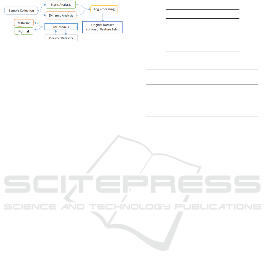
Figure 1: System Architecture.

resources(Zeltser, 2020) are Contagio malware

dump(MilaParkour, 2020), VirusShare(Mellissa,

2020) and Malwr(Community, 2017) repository. Ap-

proximately 200000 PE malware binaries have been

collected from these resources. Samples have also

been collected through malware analysis framework.

We have collected normal PE ﬁles from the win-

dows operating system and third party application

software by ﬁltering Multipurpose Internet Mail Ex-

tensions(MSDN, 2016) (MIME) type application/x-

msdownload which represents PE binary. The ﬁle size

is restricted to 3MB.

The dynamic analysis time for single binary is

approximately 5 minutes. We have used two win-

dows guest analysis environments along with single

Linux host environment. With this limited comput-

ing resources we are able to analyse two samples

in parallel(2sample/5minutes). Because of this lim-

itation, initially we are using 470 PE malware and

600 benign ﬁles for the dataset creation. A total of

1070(470+600) samples are used for the current pro-

totype experimentation. The 1070(470+600) samples

are selected randomly from the collection of mali-

cious and normal repositories respectively. The ex-

perimentation will be scaled in future for the total

sample collection by allocating more computing re-

source.

3.2 Sample Analysis and Feature

Identiﬁcation

Analysis logs of each sample is generated by perform-

ing both static and dynamic analysis. Following fea-

ture sets are identiﬁed for the dataset creation.

1. FILE META INFORMATION (Carrera, 2020;

Tek, 2020; Saxe and Berlin, 2015): is a static fea-

ture set and describes portable executable ﬁle for-

mat characteristics like entropy of sections, stack

allocation size, heap allocation size etc. This set

contains a total of 32 features which are real val-

ued. This feature set is ﬁxed and will not change

with data samples. Table 1 gives some of the ex-

ample features of this type.

Table 1: Meta Information Feature Set.

S.No. Feature

1 Size of Headers

2 Number of Sections

3 Size of Stackcommit

4 Size of Heapreserve

5 Mean Section Entropy

Table 2: Import Functions Feature Set.

S. Feature S. Feature

No. No.

1 GetProcAddress 6 ExitProcess

2 HttpOpenRequest 7 VirtualFree

3 InternetOpen 8 CreateMutex

4 GetActiveWindow 9 RegOpenKey

5 DestroyWindow 10 ShellExecute

2. IMPORT FUNCTIONS (Saxe and Berlin, 2015):

is a static feature set and describes the application

programming interface calls used by the binary

from operating system or third party software or

self contained dynamic link library. These import

functions provide information on sample charac-

teristics like network activity, system activity, per-

sistent mechanism, ﬁle system activity etc. This

set contains a total of 1805 features which are bi-

nary where value 1 indicates the feature presence

and 0 indicates the feature absence. This feature

set changes with data samples. The dimensional-

ity of this set increases with increasing data sam-

ples. We can use feature selection procedure de-

scribed in Subsection 3.3 of proposed system, to

restrict the dimensionality. Table 2 gives some of

the example features of this type.

3. Opcode Sequences (Santos et al., 2013): is a

static feature set and describes the machine in-

struction sequences present in the binary. Se-

quences of length two are considered for the

present work. Opcode sequences provides spe-

ciﬁc patterns generally malware authors use for

exploiting the vulnerabilities present in the sys-

tem. Opcode sequences also provides informa-

tion on runtime behaviour of the executables. This

feature set is huge in dimensionality. So feature

selection procedure described in Subsection 3.3

of proposed system, is applied to select the 2001

features. These features are binary where value

1 represents feature presence and value 0 repre-

sents feature absence. This feature set changes

with data samples. Table 3 provides some of the

example features.

Detection of Malicious Binaries by Applying Machine Learning Models on Static and Dynamic Artefacts

Table 3: Opcode Sequences Feature Set.

S. Feature S. Feature

No. No.

1 (PUSH, CALL) 6 (JNZ, CALL)

2 (ADD, PUSH) 7 (LEA, JMP)

3 (MOV, CALL) 8 (CMP, MOV)

4 (PUSH, JZ) 9 (XCHG, AND)

5 (XCHG, OR) 10 (ADD, CMP)

4. API Sequences (Ranveer and Hiray, 2015; Shijo

and Salim, 2015): is a dynamic feature set and de-

scribes the API call sequence the binary exhibits

upon executing it. These sequences indicate the

sample activity like ﬁle system, persistence , net-

work etc. Sequences of length two and three are

considered for the present work. Sequence set of

length 2 sequences has 373 features. Sequence set

of length 3 sequences is huge in dimensionality.

So feature selection procedure described in Sub-

section 3.3 of proposed system, is used to select

1001 features. These features are binary where

value 1 represents feature presence and value 0

represents feature absence. API sequence sets

changes with data samples. Some of the example

features are given in Tables 4,5

Table 4: API Feature Set of Length 2 Sequences.

S.No. Feature

1 (NtCreateFile, InternetConnect)

2 (WriteFile, GetForeGroundWindow)

3 (LdrLoadDll, CreateMutex)

4 (WriteFile, CreateProcess)

5 (NtCreateFile, RegSetValue)

Table 5: API Feature Set of Length 3 Sequences.

S. Feature

No.

1 (UnHookWindowHookEx, CurrentProcess, NtCreateFile)

2 (NtSetValueKey, NtCreateFile, IsUserAdmin)

3 (CreateRemoteThread, CreateThread, LdrLoadDll)

4 (WriteFile, Sleep, CreateThread)

5 (InternetConnect, NtCreateFile, HttpOpenRequest)

5. API Normal (Team, 2020a; (BusterBSA), 2020):

is a dynamic feature set and contains Operating

System API which generally are exploited to cre-

ate and execute malware with stealth and persis-

tence along with performing other malicious ac-

tivity like information gathering, network com-

promise etc. This set contains a total of 144 fea-

tures which are binary where value 1 represents

feature presence and value 0 represents feature ab-

sence. This set will not change with data samples.

Table 6: API Normal Feature Set.

S. Feature S. Feature

No. No.

1 CreateProcess 6 ShellExecute

2 HttpSendRequestEx 7 CreateMutex

3 DnsQuery UTF8 8 CreateFile

4 CreateService 9 RegDeleteKey

5 SetWindowsHookEx 10 RegSetValue

Table 6 gives some of the example features.

6. Custom Flags: is a dynamic feature set and de-

scribes the malware operational patterns. For ex-

ample a sample dropping another binary and ex-

ecuting it, which is persistent in the system, and

parent executable deletes itself is considered sus-

picious activity. This set contains 14 features

which are binary. This feature set will not change

with data samples. The description of the ﬂags is

as follows

• IMP PROCESS1. This ﬂag will be set if process

drops another payload and spans a process from

it.

• IMP PROCESS2. This ﬂag will be set if a

process spans a child process and exits it and

deletes its image.

• IMP PROCESS3. This ﬂag will be set if parent

process spans a process and moves or copies its

image location.

• IMP FILE1. This ﬂag will be set if ﬁle is

dropped and spans a process from it.

• IMP FILE2. This ﬂag will be set if a ﬁle is

dropped and adds an entry into registry for its

location.

• IMP FILE3. This ﬂag will be set if there is a

registry activity for a moved or copied ﬁle.

• IMP FILE4. This ﬂag will be set if a ﬁle is

dropped and a service is created from it.

• IMP FILE5.This ﬂag will be set if there is a ser-

vice activity for a moved or copied ﬁle.

• IMP FILE6. This ﬂag will be set if a ﬁle is

dropped and loaded into another process ad-

dress space.

• IMP FILE7. This ﬂag will be set if there is

a driver or dll loading done from a moved or

copied ﬁle.

• NETWORK. This ﬂag will be set if any network

activity is performed by the sample.

• MISC1. This ﬂag will be set if any synchro-

nization activity is performed.

• MISC2. This ﬂag will be set if binary creates

local threads or remote threads.

IoTBDS 2021 - 6th International Conference on Internet of Things, Big Data and Security

• MISC3. This ﬂag will be set if binary performs

activity like key logging etc.

3.3 Feature Selection

Some of the feature sets like opcode sequences and

API sequences have large dimensionality. We have

used Weighted Term Frequency(WTF)(Santos et al.,

2013) to select the top K features. Let us say S

, T

) is a opcode sequence of length two where

each T

is the opcode then:

W T F(S

) = T F(S

) ∗ MI(T

)

where

• T F(S

) Normalized frequency of S

• MI(T

) Mutual Information gain (Christopher

D. Manning and Sch

utze, 2008) of T

T F(S

) =

Count(S

)

∑

i=1

Count(S

)

MI(T

) = C

∗ log

N ∗ N

+ N

) ∗ (N

+ N

)

∗ log

N ∗ N

+ N

) ∗ (N

+ N

)

∗ log

N ∗ N

+ N

) ∗ (N

+ N

)

∗ log

N ∗ N

+ N

) ∗ (N

+ N

)

Count(S

). Number of occurrences of S

in total op-

code sequences.

M. Number of unique opcode sequences

N. Total opcodes frequency in all samples

P. Total opcodes frequency in malware samples

Q. Total opcodes frequency in normal samples

. T

frequency given class is Malware

. T

frequency given class is Normal

. P − N

. Q − N

3.4 Datasets

The dataset is created by taking union of all feature

sets. It has 5370 features. Three types of derived

datasets are created from the original dataset. These

derived datasets are meta datasets created by multi-

ple classiﬁers trained on individual feature sets and

combining the predictions in a speciﬁc manner. The

description of the derived datasets is as follows

• TYPE1. This dataset creation mainly focussed

on converting real valued File Meta Informa-

tion feature set from the original dataset into bi-

nary meta features. This makes the dataset uni-

form(binary) across all features. This dataset is

created by training a machine learning model on

ﬁle meta information feature set and adding pre-

diction value of each sample as b-meta feature

value for that sample. All remaining feature sets

values for each sample from the original dataset

is added without any modiﬁcation. The dimen-

sionality of this dataset is 5339. Five machine

learning models, ANN(Artiﬁcial Neural Network

Classiﬁer), KNN(K-Nearest Neighbour Classi-

ﬁer), NB(Naive Bayes Classiﬁer), RF(Random

Forest Classiﬁer) and SVM(Support Vector Ma-

chine Classiﬁer) are used for training. So ﬁve

datasets of this type are created(each one for one

speciﬁc model). Figure 2 describes the dataset

creation process. The description of the ﬁve

datasets is as follows.

1. ANN TYPE1. ANN is used for training

and prediction on real valued File Meta

Information feature set.

2. KNN TYPE1. KNN is used for training

and prediction on real valued File Meta

Information feature set.

3. NB TYPE1. NB is used for training and predic-

tion on real valued File Meta Information

feature set.

4. RF TYPE1. RF is used for training and predic-

tion on real valued File Meta Information

feature set.

5. SVM TYPE1. SVM is used for training

and prediction on real valued File Meta

Information feature set.

• TYPE2. This dataset creation mainly focused

on transforming each individual feature set from

the original dataset into a single binary feature.

The dataset is created by training machine learn-

ing models on each individual feature set sepa-

rately and concatenating the predictions for each

sample. The dimensionality of this dataset is

seven(we are using seven feature sets). Five ma-

chine learning models(ANN, KNN, NB, RF and

SVM) are used for training. So ﬁve datasets of

this type are created (each one for one speciﬁc

model). Figure 3 describes the creation process.

The description of the ﬁve datasets is as follows.

1. ANN TYPE2. ANN is used for training and

prediction on each individual feature set.

2. KNN TYPE2. KNN is used for training and

prediction on each individual feature set.

Detection of Malicious Binaries by Applying Machine Learning Models on Static and Dynamic Artefacts

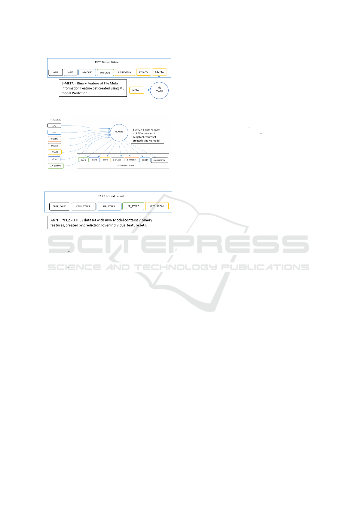
Figure 2: Type1 Derived Dataset.

Figure 3: Type2 Derived Dataset.

Figure 4: Type3 Derived Dataset.

3. NB TYPE2. NB is used for training and pre-

diction on each individual feature sett.

4. RF TYPE2. RF is used for training and predic-

tion on each individual feature set.

5. SVM TYPE2. SVM is used for training and

prediction on each individual feature set.

• TYPE3. This dataset is mainly focused on con-

catenating TYPE2 datasets of all machine learn-

ing models. The dimensionality of the dataset is

35(5 TYPE2 datasets each with seven binary fea-

tures). Figure 4 describes the dataset creation pro-

cess. For example given a sample, ANN is used

for creating 7 binary features, each one for one in-

dividual feature set. KNN is used for creating 7

binary features, each one for one individual fea-

ture set. In the same way remaining 21 features

are created using NB, RF and SVM. All these fea-

ture values concatenating together gives the data

values for the sample.

3.5 Machine Learning Models

Five machine learning models are used for this work

with conﬁgurations as given below. The performance

metric used is the classiﬁcation accuracy.

1. ARTIFICIAL NEURAL NETWORKS (Chollet,

2020; Team, 2020b):

• Two hidden layers, each with 64 units, relu ac-

tivation and 0.5 drop-out

• One output unit with sigmoid activation

• Rmsprop optimizer is used along with binary

cross entropy loss.

2. SUPPORT VECTOR MACHINES(scikit-learn

team, 2020d): Rbf kernel with parameters

C = 1.0 and gamma =

are used where d

represents number of features

3. RANDOM FOREST(scikit-learn team, 2020c):

ten estimators(trees) are used in the forest with

gini impurity criterion. The nodes are ex-

panded until all leaves becomes pure or until all

leaves contain less than 2 samples.

4. NAIVE BAYES(scikit-learn team, 2020a): Gaus-

sian Naive Bayes algorithm is used where likeli-

hood of the features are assumed to be Gaussian.

5. K-NEAREST NEIGHBOUR(scikit-learn team,

2020b): nearest Neighbour with K = 3 is used for

the classiﬁcation.

4 RESULTS

The experiment used 10-fold cross validation over

100 iterations. The classiﬁcation accuracy is taken as

average accuracy of 100 iterations. Table 7 provides

the accuracy of each classiﬁer with respect to individ-

ual feature sets. Table 8 provides the accuracy with

respect to derived datasets. The standard devia-

tion over 100 iteration across all datasets(both indi-

vidual feature sets and derived datasets) with all ma-

chine learning models is negligible. It clearly indi-

cates that the model learning is good.

The bar chart in Figure 5 describes the perfor-

mance comparison of the machine learning models

across individual feature sets. Classiﬁers performance

with respect to File Meta Information feature set is

low compared to other feature sets except for clas-

siﬁers KNN and RF. Random Forest performance is

good on average across all individual feature sets.

This is expected as the result is an ensemble of mul-

tiple estimators. Import Functions and API Se-

quences of length 3 accuracy is good across all clas-

siﬁers compared to other feature sets. ANN achieves

around 90 percent accuracy with these two feature

sets. Naive Bayes classiﬁer performance is poor over

majority of the feature sets. ANN performance is

good across majority of the feature sets.

IoTBDS 2021 - 6th International Conference on Internet of Things, Big Data and Security

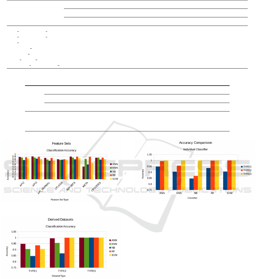
Table 7: Classiﬁcation with Individual Feature Sets.

CLASSIFIER (ACCURACY)

DATA ANN KNN NB RF SVM

SET AVG STD AVG STD AVG STD AVG STD AVG STD

API SEQUENCE 2 0.8825 0.0046 0.8617 1.1e-16 0.7589 1.1e-16 0.8716 0.0045 0.8215 4.4e-16

API SEQUENCE 3 0.9031 0.0032 0.8636 0 0.8168 0 0.8919 0.0047 0.8056 1.1e-16

API NORMAL 0.8442 0.0038 0.7785 2.2e-16 0.7308 3.3e-16 0.8407 0.0043 0.7355 1.1e-16

CUSTOM FLAGS 0.7909 0.0012 0.7664 1.1e-16 0.7748 1.1e-16 0.7897 0.0019 0.7729 1.1e-16

IMPORT FUNCTIONS 0.8986 0.0046 0.8598 2.2e-16 0.7888 1.1e-16 0.8954 0.0057 0.8383 2.2e-16

FILE META INFO 0.5036 0.0179 0.8084 3.3e-16 0.5850 0 0.8906 0.0070 0.6598 2.2e-16

OPCODE SEQUENCE 2 0.8542 0.0234 0.8579 1.1e-16 0.7766 0 0.8562 0.0064 0.8028 2.2e-16

Table 8: Classiﬁcation with Derived Datasets.

CLASSIFIER (ACCURACY)

DATA ANN KNN NB RF SVM

SET AVG STD AVG STD AVG STD AVG STD AVG STD

TYPE1 0.9481 0.0049 0.9047 1.1e-16 0.8467 1.1e-16 0.9357 0.0058 0.9056 4.4e-16

TYPE2 0.9944 1.7e-10 0.9561 2.2e-16 0.8692 2.2e-16 0.9984 0.0008 1 0

TYPE3 0.9995 0.0005 0.9991 2.2e-16 1 0 0.9998 0.0004 1 0

Figure 5: Accuracy With Individual Feature Sets.

Figure 6: Accuracy With Derived Datasets.

The bar chart in Figure 6 gives the performance com-

parison of the derived datasets across all classiﬁers.

The performance of derived datasets is better than the

performance of all individual feature sets as expected

across all machine learning models. The classiﬁca-

tion accuracy of TYPE2 derived dataset is better than

that of TYPE1 derived dataset and TYPE3 derived

dataset gives the best performance. It can be seen that

Figure 7: Accuracy Comparison over Derived Datasets for

Machine Learning Models.

TYPE3 dataset performance is very good across all

classiﬁers. TYPE3 achieves more than 99 percent ac-

curacy across all classiﬁers.

The bar chart in Figure 7 gives the performance

comparison of machine learning models across all de-

rived datasets. ANN performs well over all three de-

rived datasets. ANN, RF and SVM achieve more than

99 percent accuracy with TYPE2 and TYPE3 datasets.

Naive Bayes performance is poor with TYPE1 and

TYPE2 datasets. However it achieves 100 percent ac-

curacy with TYPE3 dataset. KNN achieves more than

90 percent accuracy across all the derived datasets.

Machine learning models provide good results

when datasets contain quality features. Providing new

information to the models always yields better results.

Most of the relevant work used limited feature sets

like combination of opcode sequences and API se-

quences or API sequences and strings etc. Our work

has used four additional feature sets along with op-

Detection of Malicious Binaries by Applying Machine Learning Models on Static and Dynamic Artefacts

code sequences and API sequences to improve the

classiﬁcation accuracy. Work on this problem done

earlier, experimented with single dataset which is a

direct combination of the feature sets. We have intro-

duced derived datasets where multi level classiﬁcation

is performed, which greatly improves the classiﬁca-

tion accuracy. With these improvements our model

classiﬁcation accuracy is more than 99.90% which is

better than existing approaches where P. V. Shijo and

A. Salim(Shijo and Salim, 2015) achieved 98.7% ac-

curacy in their work titled Integrated static and dy-

namic analysis for malware detection and Igor San-

tos et al.(Santos et al., 2013) achieved 96.60% accu-

racy in their work titled OPEM: A Static-Dynamic Ap-

proach for Machine-learning-based Malware Detec-

tion.

5 CONCLUSION

In this paper we have presented detection of ma-

licious windows binaries with behavioural analysis

along with machine intelligence approaches. Fea-

ture sets like API sequences, opcode sequences, ﬁle

meta information, custom attributes and import func-

tions are extracted from the binaries and the dataset

is created by taking the union of these feature sets.

All feature sets except ﬁle meta information are bi-

nary. File meta information is a real valued feature

set. The derived datasets are created by different

mechanisms like direct concatenation of all individual

feature sets except real valued ﬁle meta information

where machine learning models are used to make it a

single binary feature, concatenation of individual fea-

ture set predictions by machine learning model pre-

viously trained on it and, concatenation of individual

feature set predictions across all ﬁve classiﬁers pre-

viously trained on it. The results show that derived

datasets give better performance as compared to us-

ing individual feature sets. In the derived datasets,

TYPE3 dataset outperforms the other datasets. In this

work we have used four additional feature sets besides

opcode sequences and API sequences along with clas-

siﬁer ensemble methods to improve the classiﬁer per-

formance which further leads to improvement in the

malware detection rate by reducing the false positives.

We have achieved more than 99.90% classiﬁcation ac-

curacy with our work. In future, we are planning to

extend this mechanism to other ﬁle formats like MS

ofﬁce Suite and PDF etc. We are also planing to use

unsupervised and soft computing mechanisms for au-

tomatic feature extraction and selection.

6 FUTURE WORK

In this paper we have discussed detection of mali-

cious windows binaries only. This mechanism will be

extended to other ﬁle formats like Microsoft Ofﬁce

documents(Word, Power Point, Excel), Portable Doc-

ument Format(PDF) and Web Application(HTML,

HTA, JS). We are also planning to extend this mecha-

nism to other operating systems(Linux, MacOS) by

developing appropriate automatic malware analysis

engines. We are also planning to create and experi-

ment with another type of dataset known as Malware

Instruction Set(MIST Dataset ) discussed by Konrad

Reick et al.(Rieck et al., 2011) with modiﬁcations to

number of levels and argument blocks based on out-

put format of automated malware analysis framework.

We are also planning to use unsupervised models like

Latent Dirichlet allocation(LDA)(Blei et al., 2003) to

automatically extract features from analysis logs. Soft

computing techniques will be used for feature selec-

tion and weighting.

REFERENCES

Blei, D. M., Ng, A. Y., and Jordan, M. I. (2003). La-

tent dirichlet allocation. J. Mach. Learn. Res.,

3(null):993–1022.

(BusterBSA), P. L. (2020). Buster Sandbox Analyser. http:

//bsa.isoftware.nl/.

Carrera, E. (2020). peﬁle - Multi-platform Python module

to parse and work with Portable Executable (PE) ﬁles.

https://github.com/erocarrera/peﬁle.

Chollet, F. (2020). Keras: The Python Deep Learn-

ing library - The Sequential model. https://keras.io/

getting-started/sequential-model-guide/.

Christopher D. Manning, P. R. and Sch

utze, H. (2008).

Introduction to Information Retrieval, chapter 13.5.

Cambridge University Press.

Community, C. S. (2017). Malwr (Free malware analysis

service). https://malwr.com/.

Dabah, G. (2020). Powerful Disassembler Library For

x86/AMD64. https://github.com/gdabah/distorm.

Goppit (2006). Portable executable ﬁle format – a re-

verse engineer view. CodeBreakers Magazine (Se-

curity & Anti-Security- Attack & Defense), 1 issue

2. http://index-of.es/Windows/pe/CBM 1 2 2006

Goppit PE Format Reverse Engineer View.pdf.

Hunt, G. and Brubacher, D. (1999). Detours: Binary inter-

ception of win32 functions. In Third USENIX Win-

dows NT Symposium, page 8. USENIX.

Mellissa (2020). VirusShare (Repository of malware sam-

ples). https://virusshare.com/.

Michael Ligh, Steven Adair, B. H. and Richard, M. (2010).

Malware Analyst’s Cookbook and DVD: Tools and

Techniques for Fighting Malicious Code. Wiley Pub-

lishing.

IoTBDS 2021 - 6th International Conference on Internet of Things, Big Data and Security

MilaParkour (2020). Contagio (Malware Dump). http://

contagiodump.blogspot.com/.

MSDN (2016). MIME Type Detection in Windows Internet

Explorer. https://msdn.microsoft.com/en-us/library/

ms775147(v=vs.85).aspx.

Mullins, D. P. (2017). Introduction to Comput-

ing. http://cs.sru.edu/

∼

mullins/cpsc100book/

module05 SoftwareAndAdmin/module05-04

softwareAndAdmin.html.

Ranveer, S. and Hiray, S. (2015). Svm based effective mal-

ware detection system. International Journal of Com-

puter Science and Information Technologies(IJCSIT),

6(4):3361–3365.

Rieck, K., Trinius, P., Willems, C., and Holz, T. (2011). Au-

tomatic analysis of malware behaviour using machine

learning. Journal of Computer Security, 19(4):639–

668.

Santos, I., Devesa, J., Brezo, F., Nieves, J., and Bringas,

P. G. (2013). Opem: A static dynamic approach for

machine learning based malware detection. Proceed-

ings of International Conference CISIS 12-ICEUTE

12 Special Sessions Advances in Intelligent Systems

and Computing, 189:271 – 280.

Saxe, J. and Berlin, K. (2015). Deep neural network based

malware detection using two dimensional binary pro-

gram features. arXiv:1508.03096v2.

scikit-learn team (2020a). Naive Bayes. http://scikit-learn.

org/stable/modules/naive bayes.html.

scikit-learn team (2020b). Nearest Neighbors. http://

scikit-learn.org/stable/modules/neighbors.html.

scikit-learn team (2020c). RandomForestClassiﬁer.

http://scikit-learn.org/stable/modules/generated/

sklearn.ensemble.RandomForestClassiﬁer.html.

scikit-learn team (2020d). Support Vector Machines. http:

//scikit-learn.org/stable/modules/svm.html.

Shijo, P. V. and Salim, A. (2015). Integrated static

and dynamic analysis for malware detection. In-

ternational Conference on Information and Commu-

nication Technologies (ICICT 2014), 46:804 – 811.

https://doi.org/10.1016/j.procs.2015.02.149.

Team, C. D. (2020a). Cuckoo Sandbox - Automated Mal-

ware Analysis. https://cuckoosandbox.org/.

Team, G. B. (2020b). An open-source software library for

Machine Intelligence. https://www.tensorﬂow.org/.

Tek (2020). Malware-classiﬁcation. https://github.com/

Te-k/malware-classiﬁcation/blob/master/checkpe.py.

Vipre(ThreatTrack) (2020). ThreatAnalyzer. https://www.

vipre.com/products/business-protection/analyzer/.

Zeltser, L. (2020). Malware Sample Sources

for Researchers. https://zeltser.com/

malware-sample-sources/.

Detection of Malicious Binaries by Applying Machine Learning Models on Static and Dynamic Artefacts