
Malware Classification using Long Short-term Memory Models
Dennis Dang
a
, Fabio Di Troia
b
and Mark Stamp
c
Department of Computer Science, San Jose State University, San Jose, California, U.S.A.
Keywords:
Malware, Machine Learning, Deep Learning, LSTM, biLSTM, CNN.
Abstract:
Signature and anomaly based techniques are the quintessential approaches to malware detection. However,
these techniques have become increasingly ineffective as malware has become more sophisticated and com-
plex. Researchers have therefore turned to deep learning to construct better performing model. In this paper,
we create four different long-short term memory (LSTM) based models and train each to classify malware
samples from 20 families. Our features consist of opcodes extracted from malware executables. We employ
techniques used in natural language processing (NLP), including word embedding and bidirection LSTMs
(biLSTM), and we also use convolutional neural networks (CNN). We find that a model consisting of word
embedding, biLSTMs, and CNN layers performs best in our malware classification experiments.
1 INTRODUCTION
1.1 Overview
Malicious software (malware) are computer programs
that are created to harm a computer, computer sys-
tems or a computer user (Tahir, 2018). Malware at-
tacks can disrupt a person’s or organization’s day-to-
day use of their computer systems, steal personal or
confidential information, corrupt files or annoy users.
Malware can be categorized into different families
where the behavior of malware from one particular
family differs from that of another family. The pa-
pers (Choudhary and Sharma, 2020) and (Prajapati
and Stamp, 2021), for example, discuss the behavior
of many different malware families.
Modern malware attacks are generally facilitated
by the Internet. With the rise in the number of de-
vices that are connected to the Internet, it has be-
come more important than ever to keep our devices
safe, lest we risk loss of personal or confidential in-
formation (Choudhary and Sharma, 2020). While
many malware attacks are often annoying, some can
be life threatening. An example of the latter oc-
curred In 2017 when a ransomware
1
attack crippled
a
https://orcid.org/0000-0001-6842-2910
b
https://orcid.org/0000-0003-2355-7146
c
https://orcid.org/0000-0002-3803-8368
1
Ransomware is a type of malware that threatens to cor-
rupt, delete, publish or block the victim’s data unless a ran-
som is paid.
parts the United Kingdom’s National Health Service
(NHS) (Williams, 2018). Computer systems contain-
ing data pertaining to the health of thousands of pa-
tients were targeted across dozens of hospitals in the
UK. Hospitals were forced to pay a ransom to have
their files unlocked or risk having their files corrupted
or deleted. These attacks caused doctors and nurses
to cancel some 19,000 appointments, and they cost
the NHS £92 million. Malware is clearly a security
challenge that warrants a significant research effort.
Malware detection techniques include signature
based detection, anomaly based detection, and ma-
chine learning based detection (Tahir, 2018). Signa-
ture based detection has long been the most popular
approach to detecting malware. In a signature based
approach, each malware sample is first analyzed and
a signature is extracted, which is then used to iden-
tify the malware. A signature is typically a carefully
chosen, fixed bit string that is extracted from a mal-
ware sample. If the signature is found in another
sample, that sample is flagged as possible malware.
However, various code obfuscation and code morph-
ing techniques can easily thwart signature based de-
tection mechanisms.
An anomaly based detection system looks for ac-
tivity that falls outside the “normal” range of a com-
puter (Mujumdar et al., 2013), and such behavior is
flagged as suspicious. Anomaly based systems often
suffer from a high false positive rate. The drawbacks
of signature and anomaly based detection has moti-
vated the rise of machine learning techmiques.
Dang, D., Di Troia, F. and Stamp, M.
Malware Classification using Long Short-term Memory Models.
DOI: 10.5220/0010378007430752
In Proceedings of the 7th International Conference on Information Systems Security and Privacy (ICISSP 2021), pages 743-752
ISBN: 978-989-758-491-6
Copyright
c
2021 by SCITEPRESS – Science and Technology Publications, Lda. All rights reserved
743

Many classical machine learning algorithms have
found success in detecting malware (Sewak et al.,
2018). These algorithms include support vector ma-
chines (SVM), hidden markov models (HMM), ran-
dom forest, and naive Bayes, among many others.
Such models rely heavily on proper feature extrac-
tion from the dataset. Deep learning techniques have
also gained considerable traction—multilayer percep-
trons (MLP), convolutional neural networks (CNN),
and extreme learning machines (ELM) have all been
used with success (Jain et al., 2020). Other tech-
niques involving variants of recurrent neural networks
(RNN), such as gated recurrent units (GRU) and long-
short term memory (LSTM) models have received far
less attention in the literature (Lu, 2019).
In this research, we focus on using LSTMs
to classify malware by family. We build on the
work in (Lu, 2019) by combining various aspects of
the methodologies employed in (Athiwaratkun and
Stokes, 2017), (Zhang, 2020), and (Mishra et al.,
2019). Our dataset includes malware belonging to 20
distinct families, and we use opcode sequences as our
features. We consider five models, with each model
being successively more complex. Our first model
is the most basic consisting of only MLPs. This
model serves as a baseline from which we compare
our other LSTM models to. Our second model con-
sists of only one LSTM layer. Our third model is an
enhanced LSTM that includes an embedding layer,
similar to the model considered in (Lu, 2019). Our
fourth model replaces the LSTM layer from our sec-
ond previous model with a biLSTM layer. Finally, our
fifth model includes everything from our third model,
plus an additional one-dimension CNN layer and a
one-dimension max pooling layer. As far as we are a
aware, our fourth and fifth models have not previously
been considered in the literature.
The remainder of this paper is organized as fol-
lows. Section 2 discusses relevant previous work
and introduces the various deep learning techniques
employed in this research. Section 3 covers the
dataset, feature extraction, parameters, and so on. In
Section 4, we present our experimental results. Fi-
nally, Section 5 concludes the paper, and we mention
possible directions for future work.
2 BACKGROUND
2.1 Related Work
The authors of (Athiwaratkun and Stokes, 2017) con-
sider various models for malware classification. In
one of these models, a two stage classifier is used—
the first stage is either an LSTM or GRU which is
used to derive features for a second stage classifier
consisting of a single MLP layer. Another model uses
a single stage classifier consisting of nine CNN layers.
When trained and evaluated, both models achieved an
about 80% accuracy.
In (Zhang, 2020), the author proposes a novel
deep learning architecture that includes both a CNN
layer and an LSTM layer. This model is trained on
API call sequences. The CNN portion of the model
consists of filters of increasing size, with the output of
each filter fed into the LSTM layer. The output of the
LSTM layer is used as input to a dropout layer, with
a final fully connected layer for classification. The
output of the dense layer is the model’s prediction for
the given input. This model achieved an accuracy ap-
proaching 100%.
The authors of (Mishra et al., 2019) consider a
biLSTM based model to classify malware in a cloud-
based system. The model includes a CNN layer and is
trained on system call sequences. The authors achieve
an overall accuracy of approximately 90%. Inter-
estingly, the authors also show that substituting the
biLSTM for a regular LSTM layer resulted in worse
accuracies in almost all cases.
The author in (Lu, 2019) classifies malware us-
ing an entirely different approach from the two pa-
pers mentioned above. The work in (Lu, 2019) is
based on opcodes obtained from disassembled exe-
cutables. This research also employs word embed-
ding as a feature engineering step. Word embedding
techniques are often used in natural language process-
ing (NLP) applications. The result from word embed-
ding are fed into an LSTM layer. For malware detec-
tion, this model attains an average AUC of 0.99, while
for classification, the model achieves an average AUC
of 0.987.
2.2 Recurrent Neural Networks
In feedforward neural networks, all training sam-
ples are treated independently of each other (Stamp,
2017). Consequently, feedforward networks are im-
practical for cases where training samples depend on
previous samples. Thus, a different type of architec-
ture is needed in cases where “memory” is required,
as when training on time series or other sequential
data.
Recurrent neural networks (RNN) serve to add
memory to the network (Mikolov et al., 2011). As
illustrated in Figure 1 (a), the output in a RNN de-
pends not only on the current input, but also the
input from the past, as indicated by a feedback
ForSE 2021 - 5th International Workshop on FORmal methods for Security Engineering
744
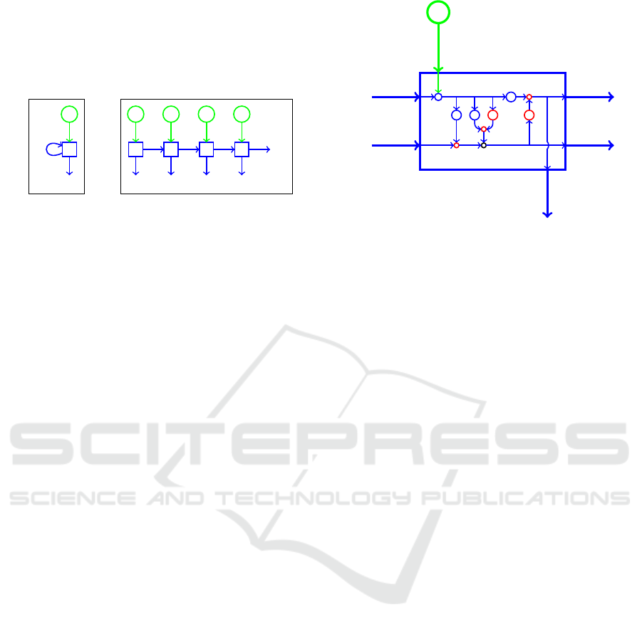
loop. Whereas information only flows forward in a
feed-forward network, information from the previous
timesteps are available at each subsequent timestep in
RNNs (Chowdhury and kashem, 2008). An unrolled
view of an RNN (Britz, 2015) appears in Figure 1 (b).
w
u
X
t
f
E
t
u
X
0
Z
0
E
0
u
w
X
1
Z
1
E
1
u
w
X
2
Z
2
E
2
u
w
X
3
Z
3
E
3
w
···
···
···
(a) Simple RNN (b) Simple RNN unrolled
Figure 1: Simple RNN and its unrolled version.
2.3 Long Short-term Memory
While conceptually simple, plain vanilla RNNs suffer
from the “vanishing gradient” issue when training via
backpropagation, which severely limits the “memory”
available to the model. To overcome this gradient
issue, complex gated RNN architectures have been
developed—the best known and most widely used
of these is long short-term memory (LSTM) models.
LSTMs address the issue of long-term dependency
by, in effect, decoupling the memory from the out-
put of the network and ensuring that additive updates
are done to the memory, rather than multiplicative up-
dates. With additive updates, the gradient is more sta-
ble.
One timestep of an LSTM is illustrated in
Figure 2. The cell state c
t
serves as a repository for
long term memory that can be tapped when needed.
The “gate” represented by W
f
enables the model to
“forget” information in the cell state, W
i
and W
g
to-
gether serve to add “memory” to the cell state, and
the structure involving the output gate W
o
allows the
model to draw on the stored memory in the cell state.
A detailed discussion of LSTMs is beyond the
scope of this paper. For more information on LSTMs,
see (Cheng et al., 2016), for example.
2.4 Bidirectional LSTM
BiLSTM models are an extension of LSTMs that pro-
cess a sequence of data in both forward and backward
directions in two separate LSTM layers. The forward
layer processes the data in the same way as a standard
LSTM, while the backward layer processes the same
data but in reverse order (Tavakoli, 2019). As with
LSTMs, a detailed discussion of biLSTMs is beyond
the scope of this paper—see, for example, (Cui et al.,
2018) for more details.
c
t−1
h
t−1
X
t
h
t
c
t
h
t
k
σ
W
o
o
t
σ
W
f
f
t
×
W
i
σ
i
t
W
g
τ
×
+
g
t
τ
×
Figure 2: One timestep of an LSTM.
2.5 Word2Vec
Word2Vec is a technique for embedding “words” into
a high-dimensional space. These word embeddings
are obtained by training a shallow neural network.
After the training process, words that are more sim-
ilar in context will tend to be closer together in the
Word2Vec space.
Perhaps surprisingly, meaningful algebraic prop-
erties also hold for Word2Vec embeddings. For ex-
ample, according to (Mikolov et al., 2013), if we let
w
0
= “king”, w
1
= “man”, w
2
= “woman”, w
3
= “queen”
and V (w
i
) is the Word2Vec embedding of word w
i
,
then V (w
3
) is the vector that is closest—in terms of
cosine similarity—to
V (w
0
) −V (w
1
) +V (w
2
)
Results such as this indicate that Word2Vec embed-
dings of English text capture significant aspects of the
semantics of the language.
In the context of this paper, the “words” are
mnemonic opcodes. We use Word2Vec embeddings
as form of feature engineering, with the Word2Vec
vectors serving as input features to our models. Pre-
vious research has shown that Word2Vec features are
more informative than raw opcode features (Chandak
et al., 2021).
2.6 Convolutional Neural Networks
Convolutional neural networks (CNNs) are de-
signed primarily to efficiently deal with local struc-
ture (Stamp, 2019). CNNs were originally designed
for use in image classification, but the technique is
applicable in any situation where some form of local
structure dominates.
Malware Classification using Long Short-term Memory Models
745

The hidden layers within a CNN act as filters
where each filter specializes in detecting a certain fea-
ture within the data, while deeper layers detect pro-
gressively more abstract features. For example, when
training on images, first layer filters might detect ver-
tical and horizontal lines, the final layer might be able
to distinguish between images of, say, dogs and cats.
While not strictly required, pooling layers can be
applied in between CNN layers. These layers re-
duce the dimensionality, thereby reducing the com-
putational load. Pooling can also reduce noise and
potentially improve performance. In max pooling, we
specify a window size and only the maximum value
within each (non-overlapping) window is retained.
2.7 TensorFlow Layers
TensorFlow models are created by adding various lay-
ers in sequence. What distinguishes one model from
another is the type of layers used and the parameters
passed into the constructors of each layer. A short de-
scription of each layer is provided below (TensorFlow
Core v.2.3.0 API, 2020).
• Input Layer: The first layer and entry point into
a neural network
• Dropout Layer: Adds noise to the network dur-
ing training by randomly severing the number of
connections between neurons from one layer to
the next. In doing so, overfitting is reduced al-
lowing models to better generalize. This typically
has the effect of increasing model accuracy during
evaluation.
• LSTM Layer: Implements a single LSTM layer
with all of the algorithms required for forward and
backward propagation.
• Bidirectional Layer: A wrapper layer that allows
RNN layers to implement bidirectional models.
Rather than implementing two separate RNN lay-
ers for the forwards and backwards direction and
concatenating the results, the bidirectional wrap-
per layer does all of this in one layer.
• Dense Layer: Implements a single fully con-
nected vanilla neural network layer.
• Embedding Layer: Responsible for mapping
positive integers to vectors of floating point val-
ues.
• Conv1D Layer: Implements the convolutional
neural network layer in one dimension.
• MaxPooling1D Layer: Implements the max
pooling operation in one dimension.
3 DATASET AND
EXPERIMENTAL DESIGN
The dataset used in this research was acquired
from (Prajapati and Stamp, 2021) and from (Nappa
et al., 2015). Our dataset consists of binary files
from 20 distinct malware families. The names of the
malware families and the number of samples per fam-
ily is shown in Table 1.
To extract features from our dataset, we first disas-
semble every executable file and extracted mnemonic
opcode sequences. Afterwards, we perform a fre-
quency analysis on all opcodes. The results from this
frequency analysis is used to sort opcodes in order
of decreasing frequency. Next, we create an opcode
to integer mapping where each opcode is assigned a
unique integer, Finally, we use this mapping to con-
vert each opcode mnemonic into integers.
We retain the 30 most frequent opcodes, with all
remaining opcodes grouped into a single “other” cate-
gory. Each omitted opcode contributes less than 0.5%
to the total number of opcodes an hence would have
minimal effect on sequence-based techniques. Note
that this approach has been used many recent stud-
ies, including (Chandak et al., 2021; Jain et al., 2020;
Prajapati and Stamp, 2021).
Table 1: Number of samples per malware family.
Malware Family Samples
Adload 1044
Agent 817
Alureon 1327
BHO 1159
CeeInject 886
Cycbot 1029
DelfInject 1097
Fakerean 1063
Hotbar
1476
Lolyda 915
Obfuscator 1331
Onlinegames 1284
Rbot 817
Renos 1309
Starpage 1084
Vobfus 924
Vundo 1784
Winwebsec 3651
Zbot 1785
Zeroacess 1119
Total 25,901
The models used in this research require all input
data to be of the same length. To accomplish this, we
experimented with various opcode sequence lengths,
as discussed below. Of course, truncating the opcode
sequence results in a loss of information, but using a
short sequence improves efficiency. Our results show
that we can obtain strong results with relatively short
ForSE 2021 - 5th International Workshop on FORmal methods for Security Engineering
746

opcode sequences.
3.1 Hardware and Software
The models used in this research were run on a
PC desktop. The specifications of this machine is
shown in Table 2. In addition, the software, operat-
ing system, and Python packages used are specified
in Table 3.
Table 2: Relevant hardware specifications.
Hardware Feature Details
CPU
Brand and Model Intel i7-8700
Base Clock Speed 3.2 GHz
# Core 6
# Threads 12
GPU
Chipset NVIDIA GeForce GTX 1070 Ti
Video Memory 8GB GDDR5
Memory Speed 1683 MHz
Cuda Cores 2432
DRAM
Brand and Model G. Skill TridentZ RGB Series
Amount 2 ×8GB = 16GB
Speed 3200MHz
Motherboard Brand and Model MSI Z370 SLI Plus LGA 1151
Table 3: Relevant software, operating system, and Python
packages.
Software Version
OS Windows 10 Pro
Python 3.8.3
Jupyter Notebook 6.1.4
Numpy 1.18.5
Scikit Learn 0.23.2
Tensorflow-GPU 2.3.1
CUDA Toolkit 10.1
cuDNN SDK 7.6
NVidia GPU Drivers 431.36
Oracle VM VirtualBox 6.0.10
VM OS Ubuntu 18.04.5 LTS
3.2 Model Parameters
Deep learning models generally have many parame-
ters that require tuning. For each of our models, we
performed a grid search over reasonable values for a
wide range of parameters—all combinations of the
values tested are listed in Table 4. All models were
trained and evaluated on the same dataset. For every
model evaluated, the accuracy was determined and
the parameters for the model with highest accuracy
were generally selected. In a few cases where ac-
curacy differences were deemed insignificant, we se-
lected parameters so that training times were reduced.
In Table 5, we list the specific values of the parame-
ters that were selected. These parameter were used for
all subsequent experiments considered in this paper.
Table 4: Parameters tested.
Parameter Values Tested
Opcode Lengths [2000, 4000, 6000, 8000, 10000]
LSTM Units [16, 32, 64, 128, 256]
Embedding Vector Lengths [16, 32, 64, 128, 256]
Dropout Amount [0.1, 0.2, 0.3, 0.4]
Table 5: Parameters selected.
Parameter Value
Batch Size 32
Maximum Number of Epochs 100
Percentage of Data to be Used in Testing 15%
Number of Unique Opcodes Used 30
Opcode Sequence Length 2000
Dropout Amount 30%
Number of LSTM Units 16
Embedding Vector Length 128
CNN Kernal Size 3
Number of CNN Filters 128
Max Pooling Size 2
3.3 Training and Testing
The dataset was sorted in ascending order based on
the number of training samples per family. The
dataset was then partitioned into four groups of five
families each, where the first group consisted of fam-
ilies with the most malware samples, while the last
group consisted of families with the least samples.
The models were trained on the first group of 5 fam-
ilies, then the second group of 10 (i.e., the first and
second groups of 5), then the third group of 15, and
finally on all families together. With each additional
group, the difficulty of classifying malware by fam-
ily increased—not only due to the inherent difficulty
of having more classes, but also due to more limited
training data for some of the families. Table 6 lists
the families that constitute each group, while Table 7
gives the number of training and testing samples for
each group considered.
The initial values of the weights of the LSTM are
randomly selected and the embedding and dense lay-
ers are randomly initialized each time the models are
trained. As a result of this random initialization, the
model will likely differ, and hence the accuracy will
also likely vary each time a model is trained. There-
fore, we train each model type on each grouping of
malware families five times. At the start of every
Malware Classification using Long Short-term Memory Models
747

Table 6: Groupings of families.
Group Malware Families
1
Hotbar
Renos
Vundo
Winwebsec
Zbot
2
Alureon
Bho
Obfuscator
Onlinegames
Zeroaccess
3
Adload
Cycbot
Delfinject
Fakerean
Startpage
4
Agent
Ceeinject
Lolyda
Rbot
Vobfus
Table 7: Number of samples for training and testing.
Groups Families
Samples
Training Testing
1 5 8480 1472
1,2 10 13,760 2400
1,2,3 15 18,272 3200
1,2,3,4 20 21,984 3872
training run, the dataset is shuffled before being split
into training and testing sets. The average of these five
cases is used to compare the different model types.
4 EXPERIMENTS AND RESULTS
In this section, we give experimental results for each
of the four model types tested. We conclude this
section with a comparison of the different models.
4.1 Using MLP Only
The structural layout of our first model using only
MLPs is given in Figure 3. Note that in this model, no
LSTMs were used. The MLP layers are represented
by dense layers. The first dense layer learns the fea-
tures of each input while the second dense layer is the
classifier. The experimental results for this model ap-
pear in Table 8. For five families, this model performs
reasonably well with average accuracy of 83.56%.
However, the accuracy drops significantly when more
families are added.
Figure 3: Structure of model using MLP only.
Table 8: Results for the MLP model.
Number of Unique
Families to Classify
Accuracy Per
Experiment (%)
Average
Accuracy (%)
5
81.95
83.56
84.08
82.41
85.14
84.21
10
56.31
57.50
56.81
59.40
61.50
53.48
15
49.27
51.22
53.18
54.82
54.54
44.31
20
53.83
50.48
45.68
52.92
46.87
53.08
4.2 LSTM without Embedding
The structural layout of our basic LSTM model given
in Figure 4. Note that the model consists of four
types layers, namely, an input layer, dropout layers,
an LSTM layer, and a dense layer. The experimental
results for this model appear in Table 9. This model
struggles with classifying just five families, with an
average accuracy of 55.73%. The accuracy drops as
more families are classified. Clearly, a more sophisti-
cated model is required.
Figure 4: Structure of LSTM model without embedding.
4.3 LSTM with Embedding
In this model, we add an embedding layer to our
basic LSTM, as illustrated in Figure 5. Note that
the embedding layer is between the input and LSTM
layer. The experimental results for this model are in
Table 10. We see a significant improvement in the ac-
curacy, with an average result of 74.66% with 5 fam-
ilies, but the accuracy drops dramatically when 10 or
more families are considered.
ForSE 2021 - 5th International Workshop on FORmal methods for Security Engineering
748
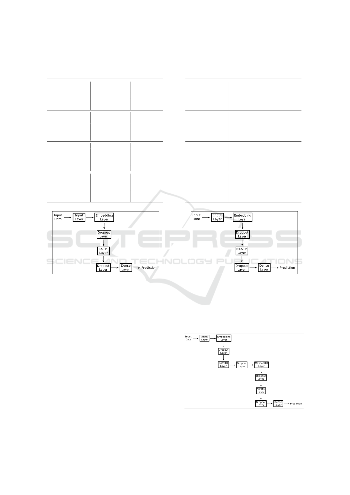
Table 9: Results for LSTM without embedding.
Number of Unique
Families to Classify
Accuracy Per
Experiment (%)
Average
Accuracy (%)
5
63.91
55.73
48.44
63.65
42.94
60.73
10
40.50
39.28
36.96
41.46
43.75
33.71
15
32.65
34.47
35.56
32.34
35.06
36.46
20
34.25
30.55
27.74
30.42
30.45
29.88
Figure 5: Structure of LSTM with embedding.
4.4 BiLSTM with Embedding
The structural layout of our first biLSTM model is
shown in Figure 6. The only difference from our pre-
vious model is that the uni-directional LSTM layer
has been replaced with a biLSTM layer. The exper-
imental results for this model are given in Table 10.
From the results, we can see that a biLSTM is far
more powerful than an LSTM in this context, as the
accuracy has improved significantly. In fact, the accu-
racy when classifying 20 families with this biLSTM
model is nearly as good as the 5-family accuracy for
the previous model.
4.5 BiLSTM with Embedding and CNN
The structure of this model appears in Figure 7. Note
that this model includes all of the layers as the previ-
ous model with the addition of a one-dimension con-
volutional layer and a max pooling layer.
Table 10: Results for LSTM with embedding.
Number of Unique
Families to Classify
Accuracy Per
Experiment (%)
Average
Accuracy (%)
5
76.09
74.66
73.64
73.17
76.90
73.51
10
54.46
54.89
56.96
55.67
54.71
52.90
15
54.28
53.36
51.97
50.28
53.22
57.03
20
51.11
49.66
52.12
51.60
45.82
47.65
Figure 6: Structure of biLSTM with embedding.
The experimental results for this case are given in
Table 12. The addition of these CNN layers improves
accuracy, and the improvement is most significant as
more families are considered—even for 20 families,
we obtained a very respectable 81.06% average accu-
racy.
Figure 7: Structure of biLSTM, embedding, and CNN
model.
Malware Classification using Long Short-term Memory Models
749
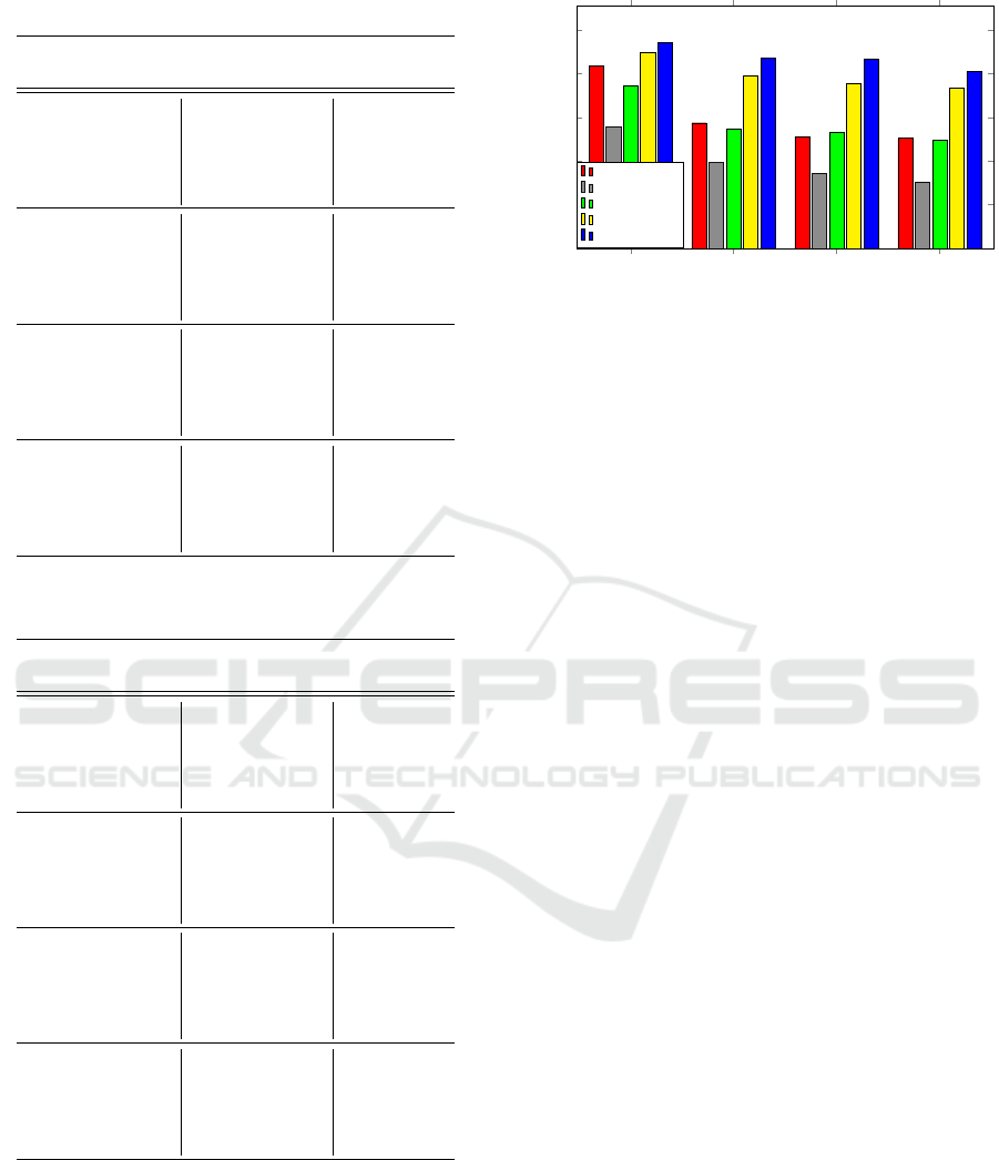
Table 11: Results for biLSTM with embedding.
Number of Unique
Families to Classify
Accuracy Per
Experiment (%)
Average
Accuracy (%)
5
89.47
89.66
90.83
89.95
85.94
92.12
10
79.58
79.30
79.54
78.13
78.79
80.46
15
76.13
75.50
76.13
76.66
76.28
72.31
20
73.71
73.36
74.74
69.53
74.10
74.72
Table 12: Results for biLSTM, embedding, and CNN
model.
Number of Unique
Families to Classify
Accuracy Per
Experiment (%)
Average
Accuracy (%)
5
93.00
94.32
96.33
92.73
94.70
94.32
10
90.42
87.38
90.29
81.29
89.58
85.29
15
87.69
86.91
87.56
82.59
87.31
89.41
20
83.29
81.06
76.34
80.60
82.18
82.88
4.6 Comparison of Results
A bar graph of the average accuracies for each model
is shown in Figure 8. As noted above, the basic
LSTM model performs poorly, with each addition to
the model improving our results.
The addition of an embedding layer dramatically
5 10 15 20
0
20
40
60
80
100
83.56
57.50
51.22
50.48
55.73
39.28
34.47
30.55
74.66
54.89
53.36
49.66
89.66
79.30
75.50
73.36
94.32
87.38
86.91
81.06
Number of Families
Accuracy (%)
MLP
LSTM
LSTM + embed
biLSTM
biLSTM + CNN
Figure 8: Comparison of the average evaluation accuracy.
increases the accuracy. This is not surprising, given
that previous work has shown that embedding layers
can greatly improve the accuracy of machine learning
models applied to opcode sequences (Chandak et al.,
2021).
BiLSTMs and word embedding are often used to-
gether in NLP applications. However , their use in
malware research appears to be very uncommon to
this point in time. Our models indicate that there is
much to be gained by considering both the forward
and backward opcode sequence.
Finally, the addition of a one-dimensional CNN
layer to the biLSTM and embedding layers gives the
best performance among the four models studied in
this research. Compared to the model without a CNN
layer, the addition of this layer seems to have greater
impact to performance when classifying more than 5
families. A possible explanation for why this model
performs so well is that in addition to the benefits that
come from having an embedding and biLSTM layers,
a CNN layer helps the model by providing a differ-
ent perspective on the opcode sequences. Specifically,
CNNs focus the model on local structure whereas the
biLSTM is focused on overall characteristics. The in-
terplay between these aspects—local and global—has
the potential to provide the best of both, which we
have married together into a single model. The addi-
tion of a max pooling layer serves to further highlight
the crucial aspects of the local structure that the CNN
highlights.
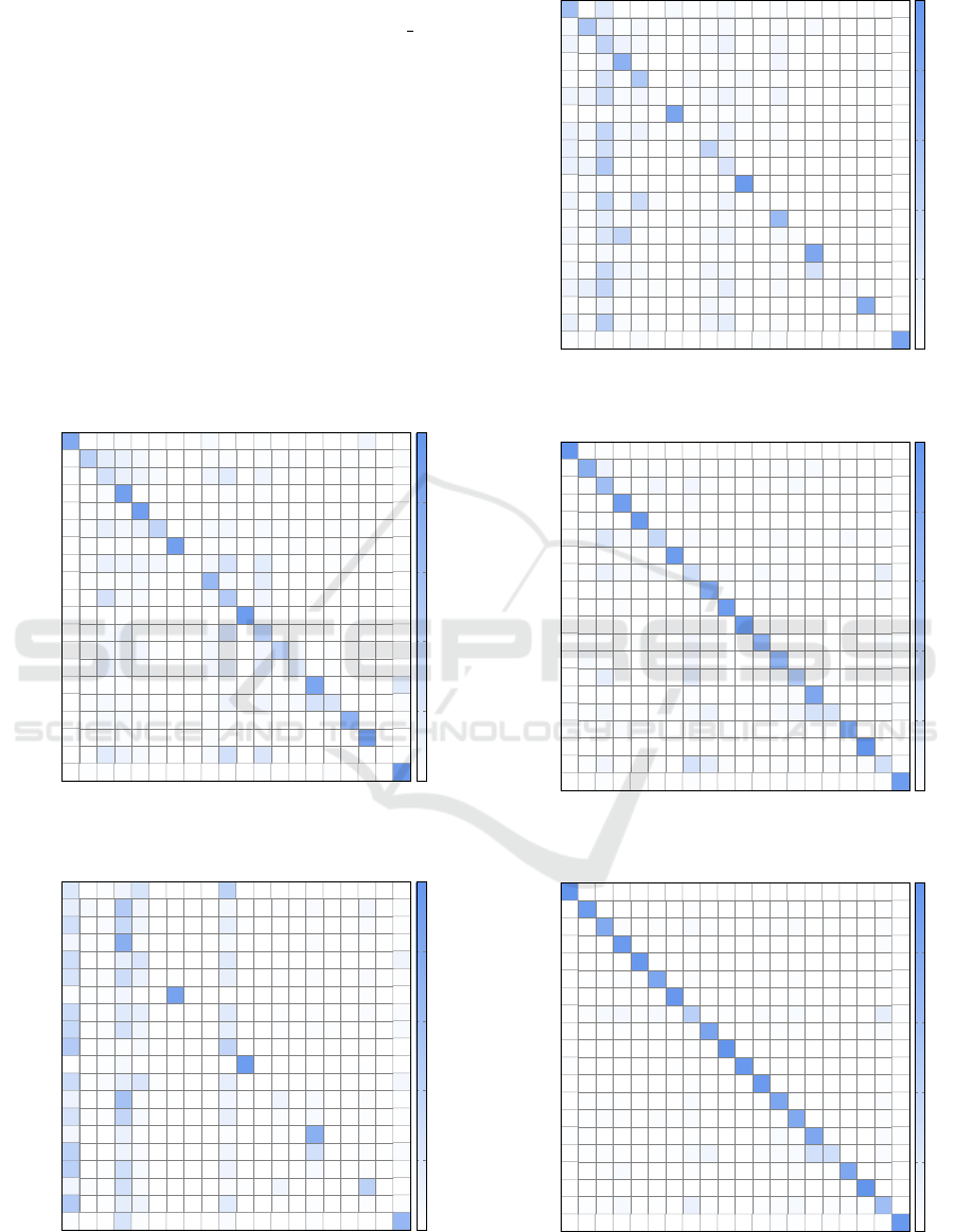
Confusion matrices for each model appear in the
Appendix in Figures 10 through 13. These matri-
ces show how often families are classified incorrectly
and precisely where these misclassifications occur.
For example, considering our best model results in
Figure 13, we see that 4 families are badly misclassi-
fied, namely, Alureon, Obfuscator, Agent, and Rbot,
with, respectively, only 36%, 31%, 25%, and 29%
classified correctly. In contrast, 8 of the families are
classified with 90% or greater accuracy.
ForSE 2021 - 5th International Workshop on FORmal methods for Security Engineering
750

5 CONCLUSION AND FUTURE
WORK
In this research, we found that malware classification
by by family using long-short term memory (LSTM)
models is feasible. However, using just a single
LSTM layer alone yields poor results. We found
that by incorporating techniques from natural lan-
guage processing (NLP), specifically, word embed-
ding and bidirectional LSTMs (biLSTM), greatly im-
proves the performance. We also discovered that that
we could get obtain even better performance by in-
cluding a convolutional neural network (CNN) layer
in our model. Our best model was able to classify
samples from 20 different malware families with an
average accuracy in excess of 81%. We conjecture
that the interplay between the long-term memory of
the biLSTM and the local structure found by the CNN
are the key to obtaining this strong performance.
For future work, more can be done into investi-
gating why applying NLP techniques are so effective
in classifying malware. The addition of an embed-
ding layer, greatly improved our model’s overall ac-
curacy. Other techniques can be considered. For ex-
ample, we might apply principle component analy-
sis (PCA) to reduce the dimensionality of the weights
obtained from the embedding layer. Additionally, ex-
periments involving different word embedding algo-
rithms (e.g., GloVe) would be worthwhile. Finally,
further research into the possible benefits of combin-
ing LSTMs and CNNs in this problem domain would
be of great interest.
REFERENCES
Athiwaratkun, B. and Stokes, J. W. (2017). Malware classi-
fication with LSTM and GRU language models and a
character-level cnn. In 2017 IEEE International Con-
ference on Acoustics, Speech and Signal Processing,
ICASSP, pages 2482–2486.
Britz, D. (2015). Recurrent neural networks tutorial,
introduction. https://www.kdnuggets.com/2015/10/
recurrent-neural-networks-tutorial.html.
Chandak, A., Lee, W., and Stamp, M. (2021). A compari-
son of word2vec, hmm2vec, and pca2vec for malware
classification. In Stamp, M., Alazab, M., and Sha-
laginov, A., editors, Malware Analysis using Artificial
Intelligence and Deep Learning. Springer.
Cheng, J., Dong, L., and Lapata, M. (2016). Long short-
term memory-networks for machine reading. https:
//arxiv.org/abs/1601.06733.
Choudhary, S. and Sharma, A. (2020). Malware detection
& classification using machine learning. In 2020 In-
ternational Conference on Emerging Trends in Com-
munication, Control and Computing, ICONC3, pages
1–4.
Chowdhury, N. and kashem, M. A. (2008). A compara-
tive analysis of feed-forward neural network recurrent
neural network to detect intrusion. In 2008 Interna-
tional Conference on Electrical and Computer Engi-
neering, pages 488–492.
Cui, Z., Ke, R., Pu, Z., and Wang, Y. (2018). Deep
bidirectional and unidirectional LSTM recurrent neu-
ral network for network-wide traffic speed prediction.
https://arxiv.org/abs/1801.02143.
Jain, M., Andreopoulos, W., and Stamp, M. (2020). Con-
volutional neural networks and extreme learning ma-
chines for malware classification. Journal of Com-
puter Virology and Hacking Techniques, 16(3):229–
244.
Lu, R. (2019). Malware detection with LSTM using opcode
language. https://arxiv.org/abs/1906.04593.
Mikolov, T., Chen, K., Corrado, G., and Dean, J. (2013).
Efficient estimation of word representations in vector
space. https://arxiv.org/abs/1301.3781.
Mikolov, T., Kombrink, S., Burget, L.,
ˇ
Cernock
`
y, J., and
Khudanpur, S. (2011). Extensions of recurrent neural
network language model. In 2011 IEEE International
Conference on Acoustics, Speech and Signal Process-
ing, ICASSP, pages 5528–5531.
Mishra, P., Khurana, K., Gupta, S., and Sharma, M. K.
(2019). Vmanalyzer: Malware semantic analysis us-
ing integrated CNN and bi-directional LSTM for de-
tecting VM-level attacks in cloud. In 2019 Twelfth In-
ternational Conference on Contemporary Computing,
IC3, pages 1–6.
Mujumdar, A., Masiwal, G., and Meshram, D. B. (2013).
Analysis of signature-based and behavior-based anti-
malware approaches. International Journal of Ad-
vanced Research in Computer Engineering and Tech-
nology, 2(6).
Nappa, A., Rafique, M. Z., and Caballero, J. (2015).
The MALICIA dataset: Identification and analysis of
drive-by download operations. International Journal
of Information Security, 14(1):15–33.
Prajapati, P. and Stamp, M. (2021). An empirical analysis of
image-based learning techniques for malware classifi-
cation. In Stamp, M., Alazab, M., and Shalaginov, A.,
editors, Malware Analysis using Artificial Intelligence
and Deep Learning. Springer.
Sewak, M., Sahay, S. K., and Rathore, H. (2018). Com-
parison of deep learning and the classical machine
learning algorithm for the malware detection. In 19th
IEEE/ACIS International Conference on Software En-
gineering, Artificial Intelligence, Networking and Par-
allel/Distributed Computing, SNPD, pages 293–296.
Stamp, M. (2017). Introduction to Machine Learning with
Applications in Information Security. Chapman &
Hall/CRC, 1st edition.
Stamp, M. (2019). Alphabet soup of deep learning topics.
https://www.cs.sjsu.edu/
∼
stamp/RUA/alpha.pdf.
Tahir, R. (2018). A study on malware and malware detec-
tion techniques. International Journal of Education
and Management Engineering, 8(2):20–30.
Tavakoli, N. (2019). Modeling genome data using bidirec-
tional LSTM. In 2019 IEEE 43rd Annual Computer
Software and Applications Conference, volume 2 of
COMPSAC, pages 183–188. IEEE.
Malware Classification using Long Short-term Memory Models
751
TensorFlow Core v.2.3.0 API (2020). Tensorflow core
v.2.3.0 api. https://www.tensorflow.org/api docs/
python/tf.
Williams, O. (2018). The WannaCry ransomware
attack left the NHS with a 73m IT bill.
https://tech.newstatesman.com/security/cost-
wannacry-ransomware-attack-nhs.
Zhang, J. (2020). Deepmal: A CNN-LSTM model
for malware detection based on dynamic semantic
behaviours. In 2020 International Conference on
Computer Information and Big Data Applications,
CIBDA, pages 313–316.
APPENDIX
Here, we provide confusion matrices for each of our
experiments in Section 4.
Hotbar
Renos
Vundo
Winwebsec
Zbot
Alureon
Bho
Obfuscator
Onlinegames
Zeroaccess
Adload
Cycbot
Delfinject
Fakerean
Startpage
Agent
Ceeinject
Lolyda
Rbot
Vobfus
Hotbar
Renos
Vundo
Winwebsec
Zbot
Alureon
Bho
Obfuscator
Onlinegames
Zeroaccess
Adload
Cycbot
Delfinject
Fakerean
Startpage
Agent
Ceeinject
Lolyda
Rbot
Vobfus
0.80 0.01 0.02 0.05 0.01
0.09
0.01 0.43 0.16 0.12 0.07 0.03 0.03 0.03 0.02 0.02 0.02 0.01 0.01 0.01 0.03
0.01 0.01 0.28 0.12 0.10 0.05
0.09
0.18 0.10 0.01 0.01 0.01 0.01 0.01
0.04
0.90
0.01 0.02 0.02
0.01 0.02 0.01
0.91
0.03 0.01
0.01 0.03 0.14 0.07 0.13
0.39
0.01 0.05 0.07 0.05 0.01 0.01 0.01 0.01 0.01 0.01
0.01 0.02
0.90
0.01 0.01 0.01 0.02 0.02
0.03 0.12
0.09 0.09
0.07 0.01 0.01 0.07 0.26 0.17 0.01 0.01 0.01 0.01 0.01 0.02
0.01 0.02 0.02 0.05 0.66 0.05 0.16
0.27 0.06 0.05 0.05
0.49
0.08
0.01 0.01
0.93
0.02 0.01
0.01 0.05 0.10 0.03 0.06 0.27 0.45 0.01
0.02 0.08 0.07 0.08 0.02 0.01 0.07 0.04 0.08 0.41 0.06 0.02 0.01 0.02
0.01 0.02 0.15 0.07 0.05 0.01 0.01 0.08 0.16 0.18 0.03 0.20 0.01 0.01 0.01
0.01 0.01 0.02 0.01 0.02 0.02 0.01 0.02 0.83 0.01 0.20
0.02 0.06 0.04 0.03 0.01 0.01 0.10
0.09
0.03 0.05 0.26 0.24 0.03
0.01 0.06 0.05 0.02 0.02 0.01 0.02 0.02 0.02 0.01 0.73 0.01 0.02
0.01 0.03 0.02 0.01 0.03
0.89
0.01 0.18 0.11 0.06 0.02 0.06
0.29
0.23 0.01 0.01 0.01 0.01 0.01
0.01 0.01 0.01 0.01 0.01
0.94
0.0
0.2
0.4
0.6
0.8
1.0
Figure 9: Confusion matrix for model using MLP only.
Hotbar
Renos
Vundo
Winwebsec
Zbot
Alureon
Bho
Obfuscator
Onlinegames
Zeroaccess
Adload
Cycbot
Delfinject
Fakerean
Startpage
Agent
Ceeinject
Lolyda
Rbot
Vobfus
Hotbar
Renos
Vundo
Winwebsec
Zbot
Alureon
Bho
Obfuscator
Onlinegames
Zeroaccess
Adload
Cycbot
Delfinject
Fakerean
Startpage
Agent
Ceeinject
Lolyda
Rbot
Vobfus
0.22 0.02
0.09
0.25 0.42
0.15 0.06 0.01
0.49
0.08 0.07 0.01 0.04 0.07 0.02
0.29
0.04 0.35
0.09
0.15 0.01 0.01 0.04 0.01
0.08 0.02 0.01 0.75 0.03 0.06 0.03 0.01 0.01
0.31 0.15 0.24 0.20 0.10
0.25 0.02 0.03 0.32 0.13 0.01 0.14 0.01 0.03 0.04 0.02
0.02 0.01 0.01 0.08 0.87 0.02
0.32 0.01 0.01 0.20 0.15 0.20 0.02 0.02 0.04 0.04
0.35 0.01 0.03 0.27
0.09
0.01 0.15 0.01 0.03 0.02 0.05
0.49
0.02 0.02 0.06
0.39
0.02
0.01 0.06
0.93
0.01
0.32 0.01 0.04 0.16 0.24 0.02 0.15 0.01 0.07
0.11 0.01 0.57 0.03 0.01 0.08 0.01 0.10 0.05 0.03 0.01
0.26 0.02 0.02 0.38 0.06 0.14 0.03 0.05 0.02 0.01
0.07 0.13 0.01 0.02 0.01 0.74 0.01
0.42 0.10 0.04
0.09 0.29
0.03 0.04
0.43 0.02 0.30 0.06 0.11 0.05 0.02 0.01
0.09
0.03 0.01 0.28 0.04 0.03 0.01
0.09
0.43
0.49
0.01 0.16 0.10 0.18 0.01 0.02 0.02 0.02
0.02 0.25 0.03 0.04 0.01 0.67
0.0
0.2
0.4
0.6
0.8
1.0
Figure 10: Confusion matrix for LSTM without embedding.
Hotbar
Renos
Vundo
Winwebsec
Zbot
Alureon
Bho
Obfuscator
Onlinegames
Zeroaccess
Adload
Cycbot
Delfinject
Fakerean
Startpage
Agent
Ceeinject
Lolyda
Rbot
Vobfus
Hotbar
Renos
Vundo
Winwebsec
Zbot
Alureon
Bho
Obfuscator
Onlinegames
Zeroaccess
Adload
Cycbot
Delfinject
Fakerean
Startpage
Agent
Ceeinject
Lolyda
Rbot
Vobfus
0.59
0.21 0.01 0.06 0.01 0.01 0.05 0.02 0.01 0.01
0.05 0.52 0.13 0.01 0.06 0.01 0.01 0.02 0.06 0.01 0.03 0.05 0.01 0.01
0.10 0.02 0.40 0.11 0.06 0.02 0.02 0.05 0.11 0.01 0.07 0.01 0.01
0.03 0.08 0.73 0.01 0.04 0.08 0.03
0.02 0.26 0.02 0.51 0.06 0.01 0.05 0.01 0.02 0.03
0.10 0.08 0.32 0.05 0.08 0.03 0.02 0.06 0.11 0.04
0.09
0.01 0.01
0.01 0.03 0.01 0.84 0.02 0.01 0.05 0.02 0.01
0.12 0.06 0.37 0.05 0.11 0.02 0.01 0.03 0.03 0.13 0.01 0.01 0.04 0.01
0.13 0.02
0.29
0.04 0.01 0.01 0.01
0.39
0.07 0.02 0.01
0.12 0.10
0.49
0.01 0.02 0.01 0.24
0.03 0.01 0.01
0.94
0.10 0.01 0.36 0.02 0.32 0.04 0.02 0.01 0.10 0.01 0.01
0.02 0.02 0.15 0.02 0.01 0.01 0.01 0.02 0.04 0.02 0.65 0.02
0.07 0.02 0.23 0.38 0.02 0.01 0.01 0.05 0.10 0.06 0.03 0.01
0.01 0.06 0.02 0.01 0.01 0.02 0.01 0.03 0.82
0.05 0.02 0.34 0.08 0.05 0.01 0.08 0.06 0.04 0.27
0.09
0.14 0.37 0.05 0.01 0.03 0.02 0.03 0.15 0.01 0.05 0.04 0.01
0.02
0.09
0.07 0.04 0.77
0.14 0.02 0.44 0.04 0.02 0.01 0.02
0.09
0.16 0.03 0.01
0.01 0.01 0.03 0.04 0.01 0.03 0.02 0.85
0.0
0.2
0.4
0.6
0.8
1.0
Figure 11: Confusion matrix for LSTM with embedding.
Hotbar
Renos
Vundo
Winwebsec
Zbot
Alureon
Bho
Obfuscator
Onlinegames
Zeroaccess
Adload
Cycbot
Delfinject
Fakerean
Startpage
Agent
Ceeinject
Lolyda
Rbot
Vobfus
Hotbar
Renos
Vundo
Winwebsec
Zbot
Alureon
Bho
Obfuscator
Onlinegames
Zeroaccess
Adload
Cycbot
Delfinject
Fakerean
Startpage
Agent
Ceeinject
Lolyda
Rbot
Vobfus
0.98
0.01 0.01
0.01 0.74 0.11 0.01 0.01 0.02 0.01 0.01 0.02 0.01 0.05
0.02 0.61 0.02 0.01 0.08 0.08 0.02 0.03 0.01 0.06 0.01 0.01 0.03
0.91
0.01 0.04 0.01 0.03
0.01 0.02
0.94
0.02 0.22 0.05 0.04 0.36 0.05 0.02 0.02 0.02 0.04 0.02 0.01 0.01 0.05 0.01 0.04 0.01
0.01 0.01
0.93
0.02 0.01
0.01 0.02 0.13 0.05 0.04 0.06 0.31 0.03 0.04 0.05 0.02 0.03 0.03 0.01 0.14 0.01
0.02 0.02 0.03 0.80 0.01 0.01 0.02 0.01 0.02 0.01 0.05
0.01 0.03 0.02
0.93
0.01 0.01 0.02
0.93
0.01 0.01
0.02 0.02 0.03 0.08 0.02 0.01 0.73 0.01 0.05 0.01
0.06 0.03 0.01 0.01 0.02 0.08 0.01 0.01 0.72 0.01 0.03
0.01 0.16 0.02 0.02 0.16 0.01 0.05 0.50 0.02 0.02 0.02
0.01 0.01 0.01 0.02 0.01 0.01 0.03 0.03 0.82 0.02 0.01
0.02 0.01 0.07 0.01 0.01 0.01 0.05 0.11 0.01 0.05 0.08 0.27 0.25 0.01 0.01 0.02
0.01 0.01 0.03 0.04 0.02 0.01 0.02 0.01 0.01 0.03 0.01 0.81
0.99
0.02 0.08 0.01 0.02 0.26 0.16 0.03 0.01 0.02 0.02 0.02 0.01 0.03
0.29
0.01
0.02 0.02 0.01 0.01
0.93
0.0
0.2
0.4
0.6
0.8
1.0
Figure 12: Confusion matrix for biLSTM with embedding.
Hotbar
Renos
Vundo
Winwebsec
Zbot
Alureon
Bho
Obfuscator
Onlinegames
Zeroaccess
Adload
Cycbot
Delfinject
Fakerean
Startpage
Agent
Ceeinject
Lolyda
Rbot
Vobfus
Hotbar
Renos
Vundo
Winwebsec
Zbot
Alureon
Bho
Obfuscator
Onlinegames
Zeroaccess
Adload
Cycbot
Delfinject
Fakerean
Startpage
Agent
Ceeinject
Lolyda
Rbot
Vobfus
0.99
0.93
0.01 0.02 0.01 0.01 0.01
0.80 0.03 0.02 0.05 0.01 0.01 0.01 0.04 0.01 0.03
0.95
0.01 0.03
0.96
0.01 0.01 0.01
0.01 0.01 0.02 0.01 0.83 0.03 0.02 0.02 0.02
0.97
0.01
0.03 0.06 0.07 0.02 0.06 0.44 0.01 0.01 0.04 0.01 0.05 0.02 0.16 0.02
0.01 0.03 0.85 0.02 0.02 0.01 0.01 0.04
0.01
0.99
0.01 0.01
0.96
0.01
0.02
0.95
0.01
0.01 0.01 0.01 0.05 0.01 0.83 0.02 0.01 0.04
0.01 0.03 0.02 0.03 0.01 0.04 0.01 0.81 0.01 0.02
0.01 0.01 0.01 0.05 0.01 0.82 0.02 0.04 0.01
0.01 0.03 0.01 0.01 0.01 0.06
0.09
0.03 0.04 0.05
0.29
0.31 0.04
0.02 0.05 0.02 0.01 0.03 0.01 0.82 0.01
1.00
0.01 0.02 0.06 0.01 0.13 0.01 0.01 0.03 0.06 0.02 0.01 0.01 0.61
0.01 0.01 0.01 0.01
0.96
0.0
0.2
0.4
0.6
0.8
1.0
Figure 13: Confusion matrix for biLSTM with embedding
and CNN.
ForSE 2021 - 5th International Workshop on FORmal methods for Security Engineering
752
