Converting Image Labels to Meaningful and Information-rich

Embeddings

Savvas Karatsiolis

and Andreas Kamilaris

Research Centre on Interactive Media, Smart Systems and Emerging Technologies (RISE), Nicosia, Cyprus

Keywords: Convolutional Neural Networks, Disentangled Latent Space, Representation Learning, Siamese Network.

Abstract: A challenge of the computer vision community is to understand the semantics of an image that will allow for

higher quality image generation based on existing high-level features and better analysis of (semi-) labeled

datasets. Categorical labels aggregate a huge amount of information into a binary value which conceals

valuable high-level concepts from the Machine Learning models. Towards addressing this challenge, this

paper introduces a method, called Occlusion-based Latent Representations (OLR), for converting image labels

to meaningful representations that capture a significant amount of data semantics. Besides being information-

rich, these representations compose a disentangled low-dimensional latent space where each image label is

encoded into a separate vector. We evaluate the quality of these representations in a series of experiments

whose results suggest that the proposed model can capture data concepts and discover data interrelations.

1 INTRODUCTION

Deep Learning (DL) advancements during the last

years offer powerful frameworks for mapping dataset

instances to binary labels and thus allow the building

of powerful classifiers for several seemingly difficult

tasks (Touvron et al., 2019), (Simonyan & Zisserman,

2015), (K. He et al., 2016), (Szegedy et al., 2017).

Classification models are usually simpler and more

successful in their task than generative models.

Likewise, transforming the instances of a dataset to

meaningful representations is harder than

transforming them into binary vectors because it

requires the preservation of data semantics.

Compressing the dataset instances into binary

numbers results in the condensation of data

interrelations to a degree that they become

undetectable and not re-constructible anymore. For

example, the value of a binary label can be calculated

by a classifier by combining the features detected

during the forward propagation of the data through

the model’s layers. At the level where the label is

calculated (i.e., the model’s output) every feature and

data characteristic has already been processed into

some high-level data abstraction. More importantly,

the high-level concepts do not contain qualitative

https://orcid.org/0000-0002-4034-7709

https://orcid.org/0000-0002-8484-4256

information or any other statistical information that

describes the degree based on which some instance

complies with a specific label. On the contrary, a label

described by a distribution instead of a binary label

mitigates the problem of blurred-out statistics and

context unawareness. The contribution of this paper

involves the investigation of suitable DL models

which allow the calculation of meaningful vectors

from the labels of a dataset with the information

provided by a classifier trained with these labels. For

this purpose, a Siamese neural network is employed,

where the information of the classifier combined with

input image occlusion enables the Siamese model to

extract discriminating features and calculate

meaningful label distributions. We call our method

Occlusion-based Latent Representations (OLR). This

work’s main contribution is a simple but effective

methodology for learning appropriate label

distributions that contain enough semantic

information and can be exploited in various ways as

demonstrated in a series of experiments. OLR builds

latent representations in a supervised manner (using

labels) that have a major advantage: latent subspaces

disentanglement. Each latent representation links

directly to one problem label and automatically

constitutes that label’s set of exclusive factors of

variation.

Karatsiolis, S. and Kamilaris, A.

Converting Image Labels to Meaningful and Information-rich Embeddings.

DOI: 10.5220/0010375801070119

In Proceedings of the 10th International Conference on Pattern Recognition Applications and Methods (ICPRAM 2021), pages 107-119

ISBN: 978-989-758-486-2

107

The rest of the paper is organized as follows:

Section 2 describes related work. Section 3 describes

the methodology followed while Section 4 presents

various experiments assessing the quality and

effectiveness of the approach. Then, Section 5

discusses the results and Section 6 concludes the paper.

2 RELATED WORK

Different studies applied a variety of strategies for

label enhancement and/or efficient separation of the

effect that each label has on the data.

2.1 Label Distribution Learning and

Label Enhancement

Hinton et al. (2015) suggested raising the temperature

coefficient of the SoftMax units at the output of the

classifier to increase the entropy of the labels’

distribution. In this way, label distribution becomes

less stringent and reveals otherwise unobservable

instance properties. Of course, this strategy can be

applied only after the model is trained and it allows

instance representation with relaxed class

probabilities, i.e., a vector containing the probability

of each class. Label distribution learning (LDL)

(Geng, 2016) aims at a similar outcome, i.e., a vector

representing the degree to which each label describes

an instance. LDL maps each instance to a label

distribution space but requires the availability of the

actual label distribution before-hand, something

which is highly impracticable in real-world

applications. Label enhanced multi-label learning

(LEMLL) (Shao et al., 2018) suggests a framework

incorporating regression of the numerical labels and

label enhancement that does not require the

availability of the label distribution. LEMLL jointly

learns the numerical labels and the predictive model

taking advantage of the topological structure in the

feature space (label enhancement).

2.2 Attribute-editing Models

Attribute-editing models are also relevant, in the

sense that they target specific attributes of the

instances. Some recent attribute-editing models

manipulate face attributes and generate images with a

set of desired (or undesired) characteristics while

preserving at the same time almost all other image

details. Given an image and the desired

characteristics (labels), an image is generated that

satisfies the given characteristics while resembling

the initial image in every other detail. Fader networks

(Lample et al., 2017) enforce an adversarial process

that makes the latent space of the labels invariant to

the attributes. Generally, the attribute-independent

latent representation is very restrictive, leading to

blurriness and distortion (Lample et al., 2017). Shen

and Liu (Shen & Liu, 2017) proposed a model that

learns the difference between images before and after

the manipulation, i.e., a residual image holding the

difference of the pixel values due to attribute-editing.

An interesting approach applying an encoder-decoder

architecture is by (Guo et al., 2019), which

compresses the original image to a latent

representation that has predefined placeholders for

the different problem classes. The model is trained

using different image pairs, editing the individual

placeholders according to the corresponding binary

labels of each image, preserving only the ones that are

set in the image label vector, and making zero every

other. Edited representations pass through the

decoder to reconstruct the original image. Besides the

two edited representations, MulGan created two more

representations by exchanging the editable

placeholders between the two representations. The

representations with the attributes exchanged pass

through a label classifier and a real/fake

discriminator. The latter uses an adversarial loss

aiming to produce more realistic images. AttGan (Z.

He et al., 2019) uses an encoder-decoder architecture

but additionally applies conditional decoding of the

latent representation based on the desired attributes

(i.e., class labels). AttGan also applies a

reconstruction, using both classification and

adversarial loss. The reconstruction preserves the

attribute-excluding details, classification loss

guarantees correct attribute manipulation while

adversarial loss aims to achieve realistic image

generation. Authors of AttGan also suggested that

symmetric skip connections between the encoder and

the decoder, like the U-Net architecture (Ronneberger

et al., 2015), improved their model’s performance.

Liu et al. (M. Liu et al., 2019) made some significant

modifications to the AttGan architecture for further

improving the results obtained. The authors of

STGAN, after conducting several experiments,

suggested that skip connections can improve the

reconstruction of the original image but at the same

time may harm attribute-editing. Their effect can be

driven to a win-win compromise using selective

transfer units that control the information flow from the

encoder to the decoder. They also suggested using a

difference attribute vector instead of the whole actual

target attribute vector (having a −1 for removing an

attribute and a +1 for adding an attribute).

ICPRAM 2021 - 10th International Conference on Pattern Recognition Applications and Methods

108

2.3 Disentangled Representations

According to Bengio (Y. Bengio, 2013), a change in

one dimension of a disentangled representation

causes a change in one variation factor while being

relatively invariant to changes in other factors.

Disentangled representations have been studied both

in the context of semi-supervised learning (Hsu et al.,

2017), (Denton & Birodkar, 2017), and unsupervised

learning (Higgins et al., 2017), (Kurutach et al.,

2018), (Kim & Mnih, 2018). Semi-supervised

approaches require knowledge about the underlying

factors of the data which is a significant limitation. β-

VAE (Higgins et al., 2017) is a disentangling

approach based on the Variational Autoencoder

(VAE) (Kingma & Welling, 2014) and achieves

latent space disentanglement by applying a slightly

different VAE objective function with a larger weight

on the Kullback–Leibler (KL) divergence between

the posterior and the prior. While the β-VAE is

appealing mainly because it relies on the elegant

framework of the VAE, it offers disentanglement to

the cost of generated image quality. Kim and Mnih

(Kim & Mnih, 2018) proposed encouraging the

VAE’s representations distribution to be factorial

which improves upon β-VAE. InfoGAN (Kurutach et

al., 2018) is a popular alternative that enhances the

mutual information between the latent codes and the

generated images.

3 METHODOLOGY

Our approach for turning the problem labels to

distributions involves the use of information from a

model trained on the classification task. Such a

classifier compresses the information of an image

down to labels and outputs probabilities of label

occurrence for an input image. We further use a

Siamese network (Neculoiu et al., 2016),(Sahito et

al., 2019),(Mueller & Thyagarajan, 2016),(Benajiba

et al., 2019) which receives two images and the

product of their label probabilities to adapt its output

𝐸 accordingly, as illustrated in Figure 1. The output

of the Siamese network

comprises L vectors of size k,

with L being the number of problem labels and 𝑒



∈

𝑅



being the row vector component of E

corresponding to label 𝑙. Effectively, the Siamese

output is a matrix holding much less information than

the original input 𝑥∈𝑅

××

, where h, w are the

height and width of the 3 channels of the image

respectively. We generally assume that 𝐿×𝑘≪ℎ×

𝑤×3. The output consists of L distributions in vector

form, one for each problem label. Since these vectors

constitute compressed representations of the input,

we will refer to them as image embeddings from this

point on.

For the Siamese model to learn the embeddings

properly, we sample pairs of images from the dataset

calculating their label probabilities using a classifier

previously trained on recognizing the labels. The

probability outcomes of the two images are multiplied

in an element-wise fashion to obtain a value for the

overall probability of each label being evident in the

image pair. Each training example comprises a triplet

of two images and the joint probability vector of their

labels (the product of the classifier’s probabilities for

the two images). The Siamese network receives the

two images of each triplet and calculates two

embeddings, one for each image. Then, it calculates

the dot products between the vector components 𝑒



the two embeddings. Assuming the two embeddings

matrices 𝐸



,𝐸



∈𝑅

×

, the dot product is calculated

between the rows of the two matrices resulting in a

vector 𝑢

⃗

∈𝑅



. The loss function of the Siamese

model is equal to the Mean Squared Error (MSE)

between 𝑢

⃗

and the joint probability vector in the

triplet. In other words, the dot product between the

label embeddings of the two images should be equal

to the joint probability vectors as calculated by the

classifier. This means that images that share a

common label should produce embeddings of the

specific class that have a high dot product.

Regarding the proposed approach, there are two

main issues to address. The first has to do with the

Siamese model architecture and the way it is designed

to have an output in the form of matrix E. The second

issue concerns the calculation of appropriate joint

probability vectors. Regarding the Siamese

architecture, after several convolutional and pooling

layers, we apply a special layer that comprises several

feature maps that form label-specific groups. The

number of groups is equal to the number of problem

labels so that each label is represented by a certain

number of feature maps 𝑘. The number of feature

maps representing a label is equal to the

dimensionality of each embedding’s vector 𝑘 and the

size of the special layer is 𝑓×𝑓×

(

𝐿×𝑘

)

, with f

being the width/height of the feature maps. At the

output of this layer, an average pooling layer is

applied which calculates the average value of each

feature map. Consequently, the output of the average

pooling layer is 𝐿×𝑘×1 and through a reshaping

operation, the output can be transformed to the

embedding’s shape L × k. The last layers of the

Siamese network are displayed in Figure 1.

Converting Image Labels to Meaningful and Information-rich Embeddings

109

The concern for calculating appropriate joint-

probability vectors is related to the classifier’s

tendency to output a high probability (close to 1) for

the correct class and a low probability (close to 0) for

the incorrect classes. This results in calculating joint

probabilities that are either close to 1 or 0 which does

not empower the Siamese model to learn the data

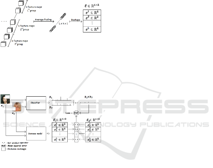
Figure 1: Final layers of the Siamese model. After several

convolutional and pooling layers, the label-specific layer

consists of L groups of k feature maps. The next layer is an

average pooling layer followed by a reshape operation

which formats the output matrix to a shape of 𝐿×𝑘, so that

there is a vector (embedding) of size k for each of the L

classes. According to the architecture, each problem label

has its feature maps which represent its statistics.

Figure 2: Training process of the Siamese model. Two

images are randomly chosen from the dataset and occlusion

rectangles are applied at random positions on them. These

rectangles are of different dimensions and have a height and

width randomly chosen from a range of values that are

between 0.33 and 0.66 of the image height and width (the

occlusion rectangles shown in the figure are smaller for

cosmetic reasons). Next, the two occluded images are

classified, and the resulting label probabilities are

multiplied to form a joint label probability. The two

occluded images and the joint probability vector form a

triplet that is used for the training of the Siamese model.

Both images go through the model and produce two image

embeddings 𝐸



,𝐸



. A dot product operation applies to the

vector components of the embeddings resulting in a vector

of L elements. The MSE between the joint probability of the

triplet (obtained from the classifier) and the dot product of

the embeddings’ vectors constitutes the loss of the training

procedure.

interrelations. The Siamese model becomes

inefficient when its training relies on over-confident

or binary vectors. Additionally, when joint

probabilities lie close to the extreme probability

values (0 or 1) the Siamese model is more prone to

overfitting and thus may not properly consider feature

correlations and interactions. Two ways for raising

the entropy of the classifier’s output were considered:

a) The first applies a strategy used in model

distillation (Hinton et al., 2015) by raising the

temperature parameter of the SoftMax function at the

output of the classifier which relaxes the label

distribution and communicates more information

about the input b) The second approach is based on

applying random partial occlusion to the input to

make the classifier less confident about its

predictions. Experiments showed that occlusion

works better in the sense that it prevents the Siamese

model from overfitting and encourages the discovery

of feature correlations and the calculation of more

expressive distributions. The degree of the occlusion

on the images of each triplet (the percentage of the

occluded image surface) can be determined

experimentally for the problem at hand. We

discovered that randomly selected occlusion

rectangles of width and height ranging from 33% to

66% of the image dimensions have a positive effect

on the training of the Siamese model. Figure 2 shows

the training process of the Siamese model.

4 RESULTS

We evaluate the proposed method on the CelebA

dataset (Z. Liu et al., 2015). The dataset contains

more than 200,000 images of faces, each annotated

with 40 binary labels (either an attribute exists or not).

Images are cropped and resized to 178 × 178 × 3

pixels. In several cases, cropping removes part of the

person’s neck thus 2 labels requiring view on the

specific (low) image region are not considered:

“wearing necklace” and “wearing necktie”. This

reduces the number of problem labels to 38.

Randomly selected 190,000 images are used in the

training set (≈ 95%) while the remaining images are

kept for the test set (≈ 5%). No pre-processing has

been applied to the images. Each label embedding has

a size of 32 which means that each image is

compressed to a representation of size 38 × 32. After

training the model and calculating the embeddings for

each image in the dataset the quality of the

embeddings is evaluated through various experiments

discussed in the following sub-sections.

ICPRAM 2021 - 10th International Conference on Pattern Recognition Applications and Methods

110

4.1 Using the Embeddings to Train a

Linear Classifier

A linear classifier was trained based on the CelebA

dataset using the calculated embeddings, to assess

their quality. The performance of the convolutional

classifier that the Siamese model relies on for its

training was used as a baseline. This comparison can

provide some useful insights on whether the

calculated embeddings are indeed capturing the data

relations. The linear classifier for this experiment has

a single layer comprising of 38 neurons representing

the classes of the dataset. Each of these neurons uses

the sigmoid activation. The embeddings calculated by

the Siamese model 𝐸∈𝑅

××

(N is the size of the

training set) are used as input to this linear model. The

linear classifier has a classification success rate of

91.6% on the test set while the convolutional

classifier has a success rate of 94.2%. This slight

performance decrease is the cost of obtaining

embeddings that capture data inter-relations, as will

be shown briefly.

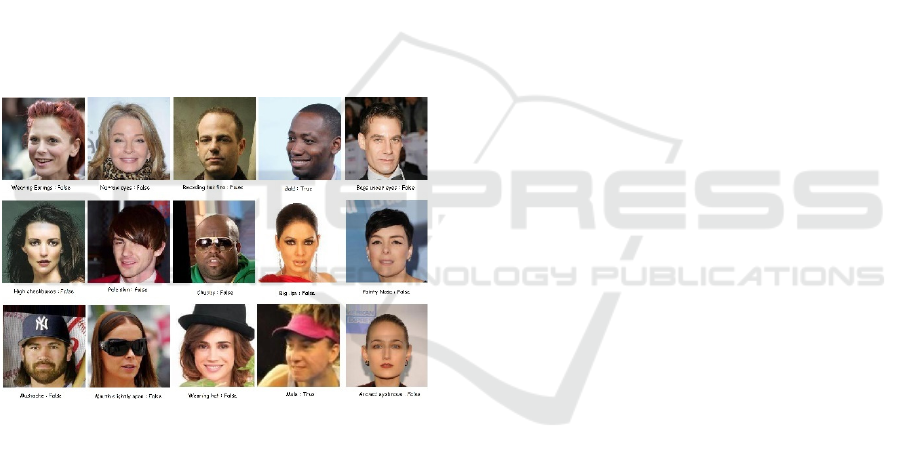
Figure 3: Examples of original CelebA images that are

accompanied by vague labels, shown under the images.

OLR does not adopt this labeling. Generally, the Siamese

embeddings are more resilient to such cases than a

convolutional classifier in the sense that they adopt a label

only if they discover strong feature correlations with other

images having the corresponding label.

The patterns classified incorrectly by the linear

model (trained on the embeddings) but, at the same

time, classified correctly by the convolutional

classifier were further analyzed. In essence, these

cases belong to the 2.6% of the test set that reflects

the success rate difference of the classifiers in

comparison. It turns out that the CelebA dataset

contains several wrong or ambiguous labels that the

Siamese embeddings did not adopt. Some examples

of questionable cases are shown in Figure 3. The

Siamese model seems to be reluctant to associate

vague labels with false evidence (features). On the

contrary, the convolutional classifier tends to learn

the ambiguous labels acting obediently in an eager to

satisfy fashion.

4.2 Correlations between the

Embeddings’ Distributions

In this experiment, the correlations between the

embeddings were examined to investigate

empirically whether the depicted label distributions

are meaningful. Figure 4 shows the Pearson

correlation coefficients between the distributions’

norm value. When a label is detected, the

corresponding embedding’s norm-value tends to

increase, reflecting the presence of such a

characteristic, otherwise, the norm-value is very

small. The high values of the vector reveal an attempt

to describe the evident label through the calculated

distribution. Some interesting and well-anticipated

correlations are revealed, for example, the positive

effect that big lips (0.3) and wearing lipstick (0.7)

may have on considering a person being attractive.

Other interesting correlations are between baldness

and attractiveness (−0.2), double chin and gray hair

(+0.5), being young and bald (−0.3), high cheekbones

and attractiveness (0.3), being male and having a big

nose (0.6), being male and having a heavy makeup

(−0.8) and the tendency to consider a smiling person

attractive (0.2). Small steps towards the pursuit of

beauty are being made here.

4.3 Principal Components Analysis of

the Embeddings’ Distribution

Principal component analysis (PCA) was applied to

the embeddings focusing on the label “Mouth slightly

open”, to further analyze the results and evaluate the

characteristics of the distribution as obtained from

OLR. This specific label was selected because almost

half of the images in the dataset contain it, hence there

is much information available for analysis. Moreover,

this label can be effortlessly detected in an image and

its detection does not rely on subjective judgment, for

example, the label regarding “attractiveness”. The

PCA applied on the “Mouth slightly open”

embeddings of all images in the dataset revealed that

the first component (eigenvector) explains 67.5% of

the data variance while the second component

explains another 4.1% of the data variance. Given the

large quantity of variance explained by the first

component, only this component was selected in this

Converting Image Labels to Meaningful and Information-rich Embeddings

111

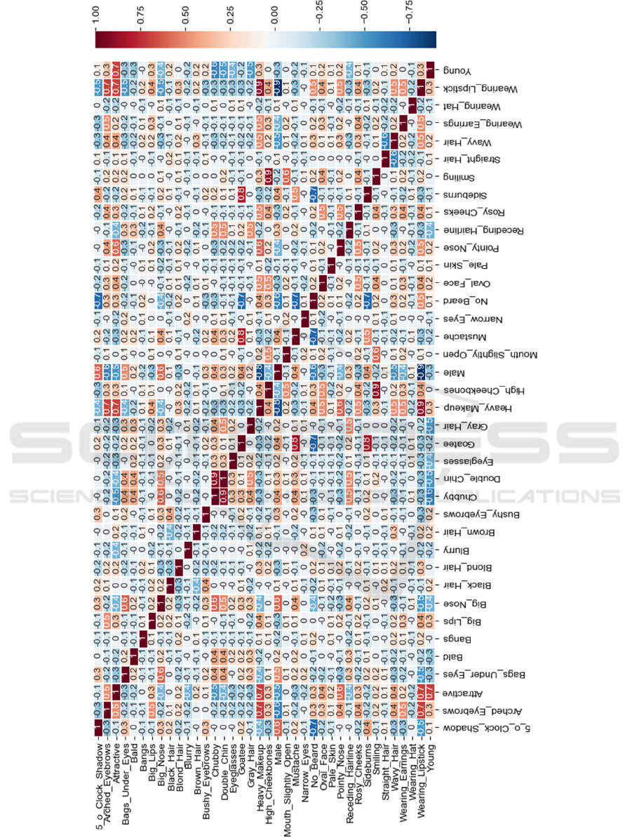
Figure 4: The Pearson correlation table between the vectors' norm value. The norm value of a specific label vector tends to

increase when a positively correlated label is evident in the same pattern. Likewise, it tends to decrease in the presence of a

negatively correlated label.

ICPRAM 2021 - 10th International Conference on Pattern Recognition Applications and Methods

112

experiment. The projections of the “Mouth slightly

open” embeddings of all images in the dataset on this

single component were sorted in increasing order of

magnitude. This results in a list of projections and

their corresponding images, starting from images that

have a smaller projection on the first principal

component moving towards images that have a larger

projection and thus comply with the selected label

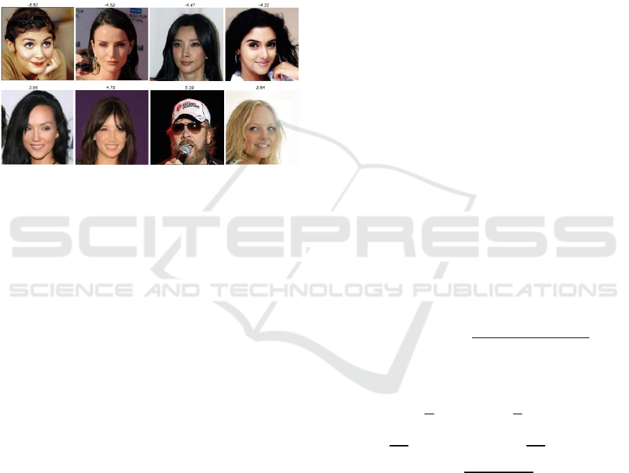
“Mouth slightly open”. Figure 5 shows some ordered

images from this experiment. A higher value of the

principal component projection signifies more

confidence in the label “open mouth” being evident.

Figure 5: Images corresponding to different projection

values of the “Mouth slightly open” embeddings on the first

principal component of the specific label’s embeddings set

(displayed in increasing order). In the top row, the images

correspond to ranking locations which are 20,000 positions

apart (ranking positions 0-80,000). From that point on,

images satisfy the “Mouth slightly open” attribute (almost

50% of the images in the dataset have the specific label).

The second row shows images corresponding to the ranking

positions 100,000-180,000. The actual projection value is

shown on top of each image.

4.4 Using the Embeddings for

Reconstructing the Images

In this experiment, each image is compressed to its

representation. If a label is evident in an image, its

corresponding vector output imprints the phenotype

of the specific label in the image. Each dataset image

has an average of eight non-zero labels, which means

that the average embeddings’ size effectively

describing an image is 8×32 = 256 out of the total

38×32 = 1216 numbers of the model’s output. The

validity of this analysis relies on the fact that any label

not evident in an image is described with a zero (or

near zero) vector, so only the active labels get a non-

zero vector value. Given the input image sizes

(178×178×3 = 95052 ), the model compresses the

input by more than 370 times, representing the images

with only 𝑝̅ ×32 numbers, where 𝑝̅ is the average

number of evident labels in the images (nonzero

labels). Due to the huge compression rate,

reconstructing the image in a way that the imprinted

face is recognized as being the same face shown in

the input image is a challenging task. The Mean

Squared Error (MSE) loss for the image

reconstruction process has some interesting

properties but also tends to create blurry images and

annoying artifacts (Wang & Bovik, 2009) (Zhao et

al., 2017). The very large compression factor applied

in the embeddings amplifies these disadvantages. The

MSE or any other norm-based distance error does not

account for the structure and the characteristics of an

image, such as the statistics among pixel values. On

the contrary, such losses produce reconstructions

which, in the general case, only approximate the raw

pixel values in the training images. A better

reconstruction could be obtained by using a loss

function that accounts for pixel statistics reflecting

the structure of the images like the structural

similarity loss function (SSIM) (Wang et al., 2004).

The SSIM loss function considers three basic image

components: luminance, contrast, and structure.

SSIM is a perceptual-based loss function that

considers some factors that are closer to what humans

perceive when they look at an image. It seems

unlikely that humans perceive an image’s content by

making pixel-level calculations in a way like what

norm-based losses do. In practice, the SSIM loss

function measures the similarity between two images

based on factors that encode the perceived change in

structural information. The SSIM between two

images x and y is calculated on various windows of

size N as follows:

𝑆𝑆𝐼𝑀

(

𝑥,𝑦

)



































































(1)

with 𝑐



and 𝑐



stabilizing the division and 𝜇



, 𝜇



, 𝜎





𝜎





and 𝜎



calculated as:

𝜇



𝑁

𝑥





, 𝜇



𝑁

𝑦





𝜎









∑(

𝑥



−𝜇



)





, 𝜎









∑

𝑦



−𝜇









𝜎



2𝜎



𝜎



+𝑐



𝜎





+𝜎





+𝑐



SSIM acts on the luma (brightness) of the images

and does not consider chrominance. For that reason,

SSIM is applied separately on each of the three color

channels of the image. To achieve even better

chromatic reconstruction, the MSE loss was also used

in conjunction with the SSIM, in a way that allows

relative freedom to each loss function’s application.

This degree of freedom is accomplished by applying

the two losses on different layers of the reconstruction

model, allowing both SSIM and MSE to operate on

different value scales. More specifically, the SSIM

Converting Image Labels to Meaningful and Information-rich Embeddings

113

loss is applied first to the output of layer Conν2D

out

which has a size of 176 × 176 × 3 as shown in Table

1. A pixel was removed from each side (top/bottom

height and left/right width) of the dataset images to

match the size of the model’s output. Next, a rescaling

layer (Rescale) puts the pixel values back to the range

y ∈ [0,1] by applying the following operation on the

output of the previous layer x:

𝑦









(



)



(



)

()

(2)

Then, the MSE loss is applied at the last layer after

the SSM loss is scaled by a factor α. The total loss

function between the reconstructed image y and the

original image x that corresponds to an input

embedding e is:

𝐿



= 𝛼 SSIM

(

𝑥,

Conv

2𝐷



)

(

1−𝛼

)

MSE

(

𝑥,𝑅𝑒𝑠𝑐𝑎𝑙𝑒

)

(3)

The reconstruction model is trained with the

RMSProp optimizer and a learning rate of 1×10



Parameter 𝑎 of equation (3) is set to 0.5. Some

reconstructions based on the test set embeddings are

shown in Figure 6 next to the original images that

produced the embeddings.

Table 1: Architecture of the reconstruction model.

Layer Output

Size (map

height,

channels)

Parameters

(kernel, channels,

stride, padding)

Flatten (1216)

Dense (18432)

Reshape (6,512)

Conv2DT (12,128) (3,128,2,same)

Conv2D (12,64) (3,64,1,same)

Conv2DT (24,64) (3,64,2,same)

Conv2D (22,64) (3,64,1,valid)

Conv2DT (44,64) (3,64,2,same)

Conv2D (44,64) (3,64,1,same)

Conv2DT (88,64) (3,64,2,same)

Conv2D (88,64) (3,64,1,same)

Conv2DT (176,64) (3,64,2,same)

Conv2D (176,32) (3,32,1,same)

Conv2D



(176,3) (3,3,1,same)

SSIM

, Conv2D



)

Rescale

(Conv2D



)

(176,3)

MSE

, Rescale)

All activation functions are ReLUs.

Input image

The reconstructions suggest that the embeddings

hold significant information from the original images,

despite the huge compression. More specifically, the

reconstructions generally tend to preserve the general

facial structure, individual characteristics, pose, and

facial expressions. This behavior is interesting for the

following reasons:

a. The reconstruction model and the Siamese

network (which is responsible for extracting

the embeddings) are separately trained with

different objective functions and there is no

co-adaptation between their tasks. However,

these models can be joined to form an implied

underdetermined autoencoder that

significantly compresses the original image to

a small internal representation (embedding)

and then decode it to reconstruct the original

image.

b. All images illustrated in Figure 6 belong to the

test set which means that the models

(embeddings’ extraction model and

reconstruction model) have never seen them

before. These images were not used during the

training of these models.

It must be noted that the image embeddings

contain significantly less information than the

original image (∼ 370 times less information). The

model maintains an important degree of similarity

between the reconstructions and the original images

despite the high compression ratio.

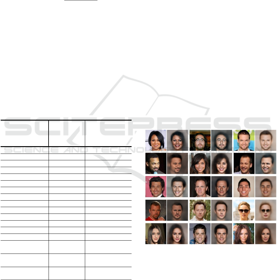
Figure 6: Several embeddings’ reconstructions compared to

the original images that produced the embeddings. Each

pair of images consists of the original image on the left and

the reconstruction on the right (3 pairs per row). Most

reconstructions tend to preserve facial structure and

characteristics, pose, and facial expression information.

The original images belong to the test set and were not used

during the training of the Siamese model or the

reconstruction model.

ICPRAM 2021 - 10th International Conference on Pattern Recognition Applications and Methods

114

4.5 Using the Embeddings for

Image-editing

Since the calculated embeddings are converted to a

distribution (or distributions of the various problem

labels), we can extract and apply inferred statistical

properties to the data. More specifically, it is assumed

that the 32-dimensional (32−d) vectors representing a

specific class (out of the 38 dataset classes) are points

on a normal probability distribution. Then, all 32−d

vectors corresponding to a specific class are used to

calculate the distribution function of the specific

problem label. For example, the embeddings’

distribution of the “wearing eyeglasses” class is

calculated from the group of images that satisfy the

specific label. Let 𝐸



be the embedding of an image

having a size of 38×32 and 𝑒





be the 32−d vector

component that corresponds to a single class 𝑙 from

the 38 classes described by the embedding. The mean

of the distribution formed by the class 𝑙 vector

components 𝑒



of all N images in the dataset that

satisfy the specific label (𝑦





= 1) is calculated by

𝜇





∑













∑

𝑒









{





}

(4)

where {.} is a qualifier function that allows

consideration only of terms that satisfy the enclosed

condition. The covariance matrix of the normal

distribution 𝛴∈𝑅

×

, where k is the vector

dimensionality (32), is calculated in a matrix form

with:

𝛴 = 𝑐𝑜𝑣



𝑋,𝑋



=𝐸

(

𝑋−𝐸



𝑋

)(

𝑋−𝐸



𝑋

)





= 𝐸



𝑋𝑋





−𝐸



𝑋



𝐸



𝑋





(5)

Approximating the distribution of each class with a

normal distribution allows drawing samples of

candidate vectors representing an instance of the

specific class. Such vectors can replace the values in

the embedding’s placeholder 𝑒





of the specific class 𝑙

in an image embedding 𝐸



. The reconstruction of the

modified embedding resembles a possible instance of

the dataset that belongs to the specific class. For

example, the embedding of an image that does not

satisfy the label “mouth slightly open” may be

modified by inserting a vector 𝑥⃗ sampled from the

embeddings’ distribution of the label “mouth slightly

open” to the placeholder 𝑒



that corresponds to the

specific label 𝑙. After making the assignment 𝑒



:=𝑥⃗,

passing the modified embedding through the

reconstruction model generates an image like the

original image which additionally satisfies the

specific label. In other words, the face in the image

remains very similar but additionally has the “mouth

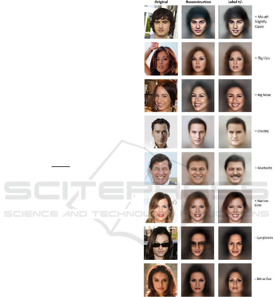
Figure 7: Examples of generating images with a property

removed or added. The original image is shown on the left

column, the reconstruction of its unmodified embedding in

the 2nd column, and the reconstruction of its modified

embedding in the 3rd column. The desired property added

or removed by modifying the embedding is shown in the

rightmost column. A plus (“+”) prefix indicates the

replacement of the appropriate embedding’s placeholder

with a vector sampled from the normal distribution of the

embeddings that satisfy the specific characteristic (label). A

minus (“-”) prefix indicates the replacement of the

appropriate embedding’s placeholder with a zero vector.

The images belong to the test set.

Converting Image Labels to Meaningful and Information-rich Embeddings

115

slightly open” property. Respectively, the phenotype

of a label can be removed by filling the embedding’s

placeholder that corresponds to the specific label with

zeros or by replacing the values of the placeholder

with a vector sampled from the distribution of the

specific label after being scaled down to a small norm

value. Vector upscaling can also be applied when

adding a specific property to an embedding by

replacing a placeholder with an upscaled vector. In

this way, the effect of adding a specific property is

increased and the phenotype change can be more

evident. Figure 7 shows several cases of sampling the

embeddings distributions for generating images with

specific characteristics or for removing specific

characteristics from images.

Interestingly, the modified embeddings generate

images of faces that are very similar to the

reconstructed images when using the original

unaltered embeddings. Additionally, the new image

has the desired characteristic added to the embedding

of the image. This experiment suggests that the 32-d

vector components of 𝑒



encode the various image

properties in an effective manner.

The degree of an edited characteristic can also be

controlled by adjusting the magnitude of the sampled

vector. For example, to add an emphasized phenotype

of a specific label to an image, the magnitude of the

sampled vector may be increased by multiplying the

vector with a scaling factor 𝑠>1. The opposite

(reduction of the vector’s magnitude) tends to add

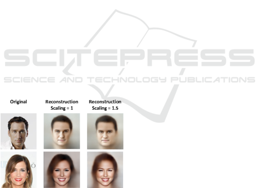
mild phenotypes. Figure 8 shows that increasing the

magnitude of the sampled vectors makes the edited

characteristic more evident.

Figure 8: The edited characteristics become more evident

when the added vector is upscaled by a certain factor to

increase its magnitude. In the first row, a vector is sampled

from the “chubby” distribution and used to edit the original

image. The rightmost image shows the result of editing the

embeddings with a vector multiplied with a scaling factor

𝑠=1.5. In the second row, the editing vector is sampled

from the “narrow eyes” distribution.

5 DISCUSSION

OLR aims to calculate the representations of each

problem label while preserving the evident label

correlations. It does not explicitly address attribute-

editing nor representing the instances in terms of

single-value class probabilities. In a sense, OLR has

some similarity with MulGan (Guo et al., 2019) in the

way specific labels get a fixed placeholder in the

latent distribution. It is different from AttGan (Z. He

et al., 2019) and STGAN (M. Liu et al., 2019) in the

sense that the latent distribution of our model

comprises solely of label representations and does not

contain any other components that encode general

image details. Essentially, OLR encodes all image

information in the label distributions while preserving

the attribute correlations. Moreover, OLR constructs

the label distributions without utilizing an adversarial,

reconstruction, or classification loss. It does this by

simply applying a supervision signal sourced from the

actual image labels. Avoiding the use of a

reconstruction loss enables the model to maintain the

correlations between the labels and to depart from

adapting according to specific image details. Various

experiments were performed (see Sections 4.1-5), to

demonstrate that OLR tends to build an understanding

of the semantics of the data distribution.

Regarding the experiment of training a linear

classifier (Section 4.1), using a dot product for

applying the labeling on the calculated features of the

Siamese model is the key operation that differentiates

OLR from the conventional way of making the

classification with a fully connected classifier

attached to a convolutional feature extractor. Usually,

the classifier consists of many neurons and accepts as

input the features detected from the preceding

convolutional layers and forms complex non-linear

relations to satisfy the output labeling. In other words,

the fully connected layers at the end of the

conventional classifier combine the calculated

features in uncontrolled and arbitrary ways under one

criterion: fitting the labels available. On the other

hand, the embeddings calculated by OLR satisfy a

probabilistic criterion: images that share labels

produce embeddings’ distributions that are similar in

the dot-product sense. The proposed method produces

label distributions that have non-zero values only if

specific features are detected in images having the

same label. In this way, the proposed approach

validates its perception of images and its decisions

regarding the conformance of each image to a label.

This conformance must be “justified” in the sense that

the compressed content vector of a specific label must

have a considerable probability of occurrence in other

ICPRAM 2021 - 10th International Conference on Pattern Recognition Applications and Methods

116

images having the same label.

The correlation results between the embeddings

(Section 4.2) suggest that OLR can calculate

embeddings that capture the relations between the

different problem labels. While these interrelations

are seemingly easy for humans to infer, establishing

these logical links is not an easy task for machine

learning (ML) models. Further, principal components

analysis on the embeddings (Section 4.3)

demonstrates that the projection on the principal

component of the embeddings’ set of each label

reflects the way the phenotype of the specific

characteristic is imprinted on the data.

Moreover, image reconstruction from the

embeddings (Section 4.4) demonstrates that the

learned representations can be transformed back to

the images that produced them. Despite the very small

size of the embeddings in comparison to the original

data and the discard of a huge amount of information,

the calculated embeddings are still able to maintain

enough information to reproduce a decent version of

the input. Finally, using the embeddings for image

editing (Section 4.5) shows that the proposed method

provides label distributions that can be exploited in

various ways for semantically-aware image editing:

an instance of a characteristic may be sampled from

the specific distribution and added to an image while

another characteristic may be removed from an image

by significantly reducing (or eliminating) the

magnitude of the respective distribution. The

phenotype of the edited characteristic (characteristic

intensity) can be controlled by modifying the

magnitude of the sampled instance.

While nothing is restraining the OLR from

working with problems that have fewer labels or a

single label per image, its full potential unravels when

dealing with problems having many labels per image.

However, despite that OLR indirectly uses labels, it

is still limited due to its reliance on supervisory

information. Another limitation arises from the fact

that, during the experiments, the image embeddings

were not allowed to adapt and were used as input data

rather than intermediate/learnable features. As such,

they did not adapt depending on the task of each

experiment and therefore they were not specialized in

tackling the specific problems. On one hand, using

unspecialized representations for a variety of tasks

stresses their quality, but on the other hand, it

produces worse results which makes the task-specific

assessment of the model more difficult. For example,

a comparison between the results of the attribute-

editing experiment (Section 4.5) and the results of

analogous models is highly unfair because our

experimental model uses embeddings that have been

learned without considering the task under study.

Future work aspires to address this limitation.

Finding a latent space in which we are fully aware

of what each variable controls, is a step forward in the

research direction of semantically-aware deep

learning and computer vision in general. OLR applies

latent space factors’ disentanglement, which is

derived from its architecture and training procedure.

Every latent representation has a non-zero magnitude

only if its respective label is evident in an image.

Occlusion-based supervision drives the model into

building representations that reflect its degree of

belief that an image complies with a label. More

importantly, these representations encapsulate image

semantics as suggested by the conditional

reconstruction experiment (Section 4.5). Converting

labels to meaningful vectors is especially useful in

many aspects. Both main ML regimes (supervised

and unsupervised learning) can benefit from

exploiting the information distilled in label

representations. As shown in the experiments

conducted, OLR builds label embeddings with

appealing properties that may be harvested by ML

methods.

In future work, we plan to add an adversarial loss

(Goodfellow et al., 2014) to the training of the

decoder to improve the quality of the reconstructed

images. Specifically, a discriminator will be added at

the output of the decoder and trained with real and

generated images. Optimization of a loss based on

both MSE and real/fake adversaries has been used

before. FSRGAN (Chen et al., 2018) uses this

technique and achieves the current perceptual state-

of-the-art in face super-resolution task for x8

upscaling. Another interesting direction would be to

modify the model for directly outputting distributions

instead of plain representations. This would resemble

variational autoencoders (Kingma & Welling, 2014)

which use a (normal) distribution for their latent

space. Converting the image labels to distributions

would be helpful for the attribute editing application

in terms of sampling an attribute point and controlling

the degree of the attribute phenotype in the generated

image (high probability samples of an attribute should

produce an emphasized attribute in the output image).

6 CONCLUSIONS

We have presented a simple method for calculating

effective representations of labels that capture the

relations among them, using a Siamese network and

a dataset of human faces. Several experiments were

conducted revealing the potential of the proposed

Converting Image Labels to Meaningful and Information-rich Embeddings

117

methodology and its ability to provide meaningful

label embeddings. The results of the experiments

suggest that the small size of the calculated

embeddings does not prevent them from maintaining

sufficient information regarding the semantics of the

data. Moreover, the experiments performed indicate

the big potential of methods that transform labels into

information-rich vectors.

REFERENCES

Benajiba, Y., Sun, J., Zhang, Y., Jiang, L., Weng, Z., &

Biran, O. (2019). Siamese Networks for Semantic

Pattern Similarity. 13th IEEE International Conference

on Semantic Computing, ICSC 2019, CA, USA, 191–

194. https://doi.org/10.1109/ICOSC.2019.8665512

Bengio, Y. (2013). Deep learning of representations:

Looking forward. Lecture Notes in Computer Science

(Including Subseries Lecture Notes in Artificial

Intelligence and Lecture Notes in Bioinformatics), 7978

LNAI, 1–37. https://doi.org/10.1007/978-3-642-39593-

2_1

Chen, Y., Tai, Y., Liu, X., Shen, C., & Yang, J. (2018).

FSRNet: End-to-End Learning Face Super-Resolution

with Facial Priors. 2018 IEEE/CVF Conference on

Computer Vision and Pattern Recognition, 2492–2501.

Denton, E., & Birodkar, V. (2017). Unsupervised learning

of disentangled representations from video. Advances

in Neural Information Processing Systems, 2017-

December, 4415–4424. http://arxiv.org/abs/1705.10

915

Geng, X. (2016). Label Distribution Learning. IEEE Trans.

Knowl. Data Eng., 28(7), 1734–1748.

Goodfellow, I., Pouget-Abadie, J., & Mirza, M. (2014).

Generative Adversarial Networks. CoRR, abs/1406.2.

Guo, J., Qian, Z., Zhou, Z., & Liu, Y. (2019). MulGAN:

Facial Attribute Editing by Exemplar. CoRR,

abs/1912.1.

He, K., Zhang, X., Ren, S., & Sun, J. (2016). Deep Residual

Learning for Image Recognition. Conference on

Computer Vision and Pattern Recognition (CVPR),

770–778.

He, Z., Zuo, W., Kan, M., Shan, S., & Chen, X. (2019).

AttGAN: Facial Attribute Editing by Only Changing

What You Want. IEEE Transactions on Image

Processing, 28(11), 5464–5478.

Higgins, I., Matthey, L., Pal, A., Burgess, C., Glorot, X.,

Botvinick, M., Mohamed, S., & Lerchner, A. (2017).

beta-VAE: Learning Basic Visual Concepts with a

Constrained Variational Framework. ICLR (Poster

Session).

Hinton, G. E., Vinyals, O., & Dean, J. (2015). Distilling the

Knowledge in a Neural Network. Computing Research

Repository (CoRR). http://arxiv.org/abs/1503.02531

Hsu, W.-N., Zhang, Y., & Glass, J. R. (2017). Unsupervised

Learning of Disentangled and Interpretable

Representations from Sequential Data. In I. Guyon, U.

von Luxburg, S. Bengio, H. M. Wallach, R. Fergus, S.

V. N. Vishwanathan, & R. Garnett (Eds.), Advances in

Neural Information Processing Systems 30: Annual

Conference on Neural Information Processing Systems

2017, 4-9 December 2017, Long Beach, CA, {USA} (pp.

1878–1889).

Kim, H., & Mnih, A. (2018). Disentangling by factorising.

In J. G. Dy & A. Krause (Eds.), 35th International

Conference on Machine Learning, ICML 2018 (Vol. 6,

pp. 4153–4171). PMLR.

Kingma, D. P., & Welling, M. (2014). Auto-Encoding

Variational Bayes. In Y. Bengio & Y. LeCun (Eds.),

2nd International Conference on Learning

Representations, ICLR 2014, Conference Track

Proceedings. http://arxiv.org/abs/1312.6114

Kurutach, T., Tamar, A., Yang, G., Russell, S., & Abbeel,

P. (2018). Learning plannable representations with

causal infogan. In S. Bengio, H. M. Wallach, H.

Larochelle, K. Grauman, N. Cesa-Bianchi, & R.

Garnett (Eds.), Advances in Neural Information

Processing Systems (Vols. 2018-Decem, pp. 8733–

8744).

Lample, G., Zeghidour, N., Usunier, N., Bordes, A.,

Denoyer, L., & Ranzato, M. (2017). Fader Networks:

Manipulating Images by Sliding Attributes. In I.

Guyon, U. von Luxburg, S. Bengio, H. M. Wallach, R.

Fergus, S. V. N. Vishwanathan, & R. Garnett (Eds.),

NIPS (pp. 5967–5976).

Liu, M., Ding, Y., Xia, M., Liu, X., Ding, E., Zuo, W., &

Wen, S. (2019). STGAN: A Unified Selective Transfer

Network for Arbitrary Image Attribute Editing. CoRR,

abs/1904.0.

Liu, Z., Luo, P., Wang, X., & Tang, X. (2015). Deep

Learning Face Attributes in the Wild. Proceedings of

International Conference on Computer Vision (ICCV).

Mueller, J., & Thyagarajan, A. (2016). Siamese Recurrent

Architectures for Learning Sentence Similarity. In D.

Schuurmans & M. P. Wellman (Eds.), AAAI (pp. 2786–

2792). AAAI Press.

Neculoiu, P., Versteegh, M., & Rotaru, M. (2016). Learning

Text Similarity with Siamese Recurrent Networks. In P.

Blunsom, K. Cho, S. B. Cohen, E. Grefenstette, K. M.

Hermann, L. Rimell, J. Weston, & S. W. tau Yih (Eds.),

Rep4NLP@ACL (pp. 148–157). Association for

Computational Linguistics.

Ronneberger, O., Fischer, P., & Brox, T. (2015). U-Net:

Convolutional Networks for Biomedical Image

Segmentation. International Conference of Medical

Image Computing and Computer-Assisted Intervention

18 (MICCAI), 234–241.

Sahito, A., Frank, E., & Pfahringer, B. (2019). Semi-

supervised Learning Using Siamese Networks. In J. Liu

& J. Bailey (Eds.), Australasian Conference on

Artificial Intelligence (Vol. 11919, pp. 586–597).

Springer.

Shao, R., Xu, N., & Geng, X. (2018). Multi-label Learning

with Label Enhancement. ICDM, 437–446.

Shen, W., & Liu, R. (2017). Learning Residual Images for

Face Attribute Manipulation. CVPR, 1225–1233.

ICPRAM 2021 - 10th International Conference on Pattern Recognition Applications and Methods

118

Simonyan, K., & Zisserman, A. (2015). Very deep

convolutional networks for large-scale image

recognition. In 3rd International Conference on

Learning Representations, ICLR 2015 - Conference

Track Proceedings.

Szegedy, C., Ioffe, S., Vanhoucke, V., & Alemi, A. A.

(2017). Inception-v4, Inception-ResNet and the Impact

of Residual Connections on Learning. In S. P. Singh &

S. Markovitch (Eds.), Proceedings of the Thirty-First

AAAI Conference on Artificial Intelligence, February

4-9, 2017, San Francisco, California, USA (pp. 4278–

4284). AAAI Press.

Touvron, H., Vedaldi, A., Douze, M., & Jégou, H. (2019).

Fixing the train-test resolution discrepancy. In H. M.

Wallach, H. Larochelle, A. Beygelzimer, F. d’Alché

Buc, E. B. Fox, & R. Garnett (Eds.), Advances in

Neural Information Processing Systems (NeurIPS) (pp.

8250–8260).

Wang, Z., & Bovik, A. C. (2009). Mean squared error: Love

it or leave it? A new look at Signal Fidelity Measures.

IEEE Signal Process. Mag., 26(1), 98–117.

Wang, Z., Bovik, A. C., Sheikh, H. R., & Simoncelli, E. P.

(2004). Image quality assessment: from error visibility

to structural similarity. IEEE Transactions on Image

Processing, 13(4), 600–612.

Zhao, H., Gallo, O., Frosio, I., & Kautz, J. (2017). Loss

Functions for Image Restoration With Neural

Networks. IEEE Trans. Computational Imaging, 3(1),

47–57.

Converting Image Labels to Meaningful and Information-rich Embeddings

119