
Applying PySCMGroup to Breast Cancer Biomarkers Discovery
Mazid Abiodoun Osseni
1 a
, Prudencio Tossou
1,2 b
, Jacques Corbeil
1 c
and Franc¸ois Laviolette
1,3 d
1
Universit
´
e Laval, Qu
´
ebec, Canada
2
InVivo AI, Montr
´
eal, Canada
3
Mila, Montr
´
eal, Canada
Keywords:
Multi-omics, Breast Cancer, Interpretability, Penalty-weight, Pathway Guided Selection.
Abstract:
Background. The identification of biomarkers associated with triple-negative breast cancer (TNBC) is still
an active area of research due to the complexity of finding robust biomarkers associated with the disease. Pre-
vious methods have attempted to tackle the problem from a mono-perspective view by analyzing each omics
individually in the search of biomarkers. The majority of these methods mainly focus on gene expression
analysis since their impact on the phenotype is easier to measure and possibly more direct. However, it is
common understanding that genes belong to pathways and tend to work together within various metabolic,
regulatory, and signalling pathways. Hence, in this work, we tackled the TNBC biomarker discovery prob-
lem as a multi-omic pathway-based problem by efficiently combining the biological knowledge from multiple
pathways using a novel machine learning algorithm. The proposed algorithm, called GroupSCM, is an exten-
sion of the Set Covering Machine (SCM) that incorporate the pathway features as priors.
Results. Although the GroupSCM performed similarly to the SCM, metric-wise, it helps identify new
biomarkers not previously found by the SCM. By leveraging the pathway priors, the GroupSCM was able
to uncover two miRNAs: hsa-mir-18a and hsa-mir-190b, already known to be associated with various cancers
including breast cancer and yet to be linked to the Triple-Negative Breast Cancer phenotype.
Conclusion. The addition of priors to the SCM leads to interpretable, complete and sparser models which
are easier to analyze in vivo settings. It also provides insight into the omics interaction by highlighting the
miRNAs and epigenome contribution to the prediction task.
Code Availability: The code is available at: https://github.com/dizam92/BRCA experiments and paper
1 INTRODUCTION
Based on their genes expression, breast cancer (BC)
cases can be sub-classified into five categories: lumi-
nal A, luminal B, HER2++, Basal like and Triple-
Negative Breast Cancer (TNBC) (Lehmann et al.,
2011). TNBC, characterized by the non-expression
of estrogen (ER), progesterone (PR), and HER2 re-
ceptors, represents 10-20% of all breast cancers and is
known to be the most aggressive form, i.e. most likely
to spread beyond the breast and recur post-treatment
(Weigelt et al., 2010). Unfortunately, TNBC still re-
mains poorly diagnosed, as clinical, microarray-based
studies and immunohistochemical profiling are often
inconclusive, due to its similarity with the basal-like
a
https://orcid.org/0000-0001-7358-7402
b
https://orcid.org/0000-0002-9841-9867
c
https://orcid.org/0000-0002-9973-2740
d
https://orcid.org/0000-0002-1937-2512
breast cancer type. Consequently, there is a need for
the discovery of additional biomarkers to improve the
clinical diagnostic and prediction prognosis between
TNBC and other breast cancer types.
Genetic studies of cancer diseases in general have
often focused on extracting information from as-
sociation analysis using only a few types of data.
For example, (Iorio et al., 2005) showed that, com-
pared with normal breast tissue, miRNAs (specifi-
cally miR-125b, miR-145, miR-21 and miR-155) are
also aberrantly expressed in human Breast Cancer.
In the case of the Colorectal Cancer (CRC), (Lao
and Grady, 2011) put more emphasis on the fact that
the hyper-methylation of some CpGs site ahead of
certain genes (CXCL12) can promote the metastatic
behaviour of colon cancer cell lines. However, to
better understand the disease’s complex genetic ex-
planation and in order to provide robust biomark-
ers, it is becoming increasingly important to inte-
72
Osseni, M., Tossou, P., Corbeil, J. and Laviolette, F.
Applying PySCMGroup to Breast Cancer Biomarkers Discovery.
DOI: 10.5220/0010375500720082
In Proceedings of the 14th International Joint Conference on Biomedical Engineering Systems and Technologies (BIOSTEC 2021) - Volume 3: BIOINFORMATICS, pages 72-82
ISBN: 978-989-758-490-9
Copyright
c
2021 by SCITEPRESS – Science and Technology Publications, Lda. All rights reserved

grate and utilize the full scope of available omics
information, recorded from a wide range of exper-
imental modalities (Freedman et al., 2011), (Kar-
czewski and Snyder, 2018). Embracing this philos-
ophy, numerous studies combined omics to tackle
the biomarkers discovery problem. Using unbiased
multi-omics approaches, (Yuan et al., 2016) reported
that DNA topoisomerase 2 beta (TOP2B) shows a
male-biased difference in DNA methylation in Blad-
der Cancer. In the case of Calcific Aortic Valve Dis-
ease (CAVD), (Heuschkel et al., 2020) demonstrated
that the multi-omics integration of overlapping pro-
teome/transcriptome molecules, with the miRNAs,
identified a CAVD protein–protein interaction net-
work. Meanwhile (Rappoport et al., 2020) introduced
MONET (Multi Omic clustering by Non-Exhaustive
Types) aimed at discovering modules of similar sam-
ples such that each module is allowed to have a
clustering structure for only a subset of the omics.
This is a multi-omics clustering approach which dif-
fers from the other algorithms by not assuming a
common structure across all omics data. (Delogu
et al., 2020) proposed that upgrading multi-omics
toolkits with traditional absolute measurements un-
locks the scaling of core biological questions to dy-
namic and complex microbiomes, creating a deeper
insight into inter-organismal relationships that drive
the greater community function. (Bareche et al.,
2018) used copy-number aberrations, somatic muta-
tions and gene expression data to demonstrate the
substantial genomic heterogeneity that characterizes
TNBC molecular subtypes, allowing for a better un-
derstanding of the disease biology as well as the iden-
tification of several candidate targets paving novel ap-
proaches for the development of anticancer therapeu-
tics for TNBC. (Singh et al., 2016) presented DIA-
BLO (Data Integration Analysis for Biomarker dis-
covery using a Latent component method for Omics
studies) a multivariate analysis method based on the
dimension reduction maximizing the correlation be-
tween each omics pairs. It underlines the importance
of the processing of the interaction between omics
data before using them for the prediction task.
Following this trend towards the integration of
multi-omics data this work presents a machine learn-
ing algorithm based on pathways interactions be-
tween gene expression, epigenome expression and
miRNAs expression to learn interpretable and sparse
models uncovering potentially new candidate targets
for the development of anticancer therapeutics for
TNBC. The use of the multi-omics data helps empha-
sis the interaction between the different omics which
leads to a better interpretation of the mechanism so-
lution. Here we focus on the interpretable model
because we strive to explain why these features are
selected in the model decision path. There are two
types of models in machine learning, generally speak-
ing: the black box model and the interpretable model.
An interpretable machine learning refers to methods
and models that make the behaviour and predictions
of machine learning systems understandable to hu-
mans. It differs from the black box model which
is a system that does not reveal its internal mecha-
nisms. Interpretability is more of a concept there-
fore there is no real mathematical definition of inter-
pretability. A (non-mathematical) definition reported
by (Miller, 2019) is: Interpretability is the degree to
which a human can understand the cause of a deci-
sion. The need for interpretability here lies in the fact
that for some tasks (especially the biological data), it
is not enough to get the prediction (the what) (Doshi-
Velez and Kim, 2017). The model must also explain
how it came to the prediction (the why), because a
correct prediction only partially solves your original
problem (Molnar, 2019). Moreover, interpretability
favours the acceptance of the model by health practi-
tioners. Before the learning phase, there is a need to
integrate the omics data. (Ritchie et al., 2015) define
the integration of omics as the combination of multi-
ple omics datasets to develop multivariate models to
predict complex phenotypes. Mainly, it is the con-
catenation method (Liu et al., 2013) and the ensem-
ble method (G
¨
unther et al., 2012). The concatenation
method consists of putting all the omics together i.e.
side-by-side and treating them as only one mega-set.
The ensemble method consists of learning a classifier
on each omics dataset and building a majority vote
with the classifiers, for the final prediction. With time,
new methods were also explored including the clus-
tering (Rappoport et al., 2020) and the graph network
((Singh et al., 2016), (Heuschkel et al., 2020)). Here,
in this work, the goal is to let the algorithm infer po-
tential interaction between the features with the inte-
gration of new priors based on pathways of gene inter-
actions. Therefore the concatenation method which
does not imply any priors on the feature is more suit-
able for the task at hand. Depending on what a feature
refers to, pathway-based feature selection methods
can be classified into three categories: pathway-level
selection, bi-level selection and pathway-guided gene
selection (Tian et al., 2019). In the pathway-level se-
lection, the goal is to select the whole pathways as-
sociated with the phenotypes of interest ((Dinu et al.,
2007), (Wu et al., 2010)). The bi-level selection is a
process, which identifies not only relevant pathways
but also important genes that contribute critically to
the significance of identified relevant pathways. In the
pathway-guided gene selection, a feature corresponds
Applying PySCMGroup to Breast Cancer Biomarkers Discovery
73

to an individual gene.
The algorithm (GroupSCM) presented here is
an extension of the Set Covering Machine (SCM)
which was originally introduced by (Marchand and
Shawe-Taylor, 2002). The SCM is a learning algo-
rithm using a greedy approach to learn a conjunc-
tion set or a disjunction set of rules. The rules are
the decision stumps (omic value expression ≤ v or
omic value expression ≥ v). The SCM applicability
to the biomarker discovery task world is an effective
algorithm in the domain. Kover (Drouin et al., 2016),
a software used in the prediction of antibiotic resis-
tance in bacteria is based on the SCM. This a robust
algorithm yields great results in the antibiotic resis-
tance prediction problem in accordance with the pub-
lished literature. The GroupSCM extends the classi-
cal SCM to integrate the knowledge of variables in-
teracting in biological pathways. The intuition behind
this is to favour a rule selection based on their path-
ways association. The GroupSCM use the pathway-
guided gene selection as priors and modify the utility
function of the SCM into taking in account different
weights on each feature depending on the pathways to
which they belong.
2 METHODS
Let’s S be a set of data such as S
def
=
{
(x
i
, y
i
)
}
m
i=0
∼ D
m
where x
i
∈ X is a training example, y
i
∈ Y its asso-
ciated label, D is a data generating distribution and
m the size of the dataset. In this work, we consider
the diagnosis of TNBC for a patient as a binary clas-
sification task where x
i
represents the ith patient data
(multi-omics features) and y
i
∈
{
−1, 1
}
whether the
patient is TNBC or non-TNBC. Below we first de-
scribe the original SCM algorithm then we present
our extension, the GroupSCM.
2.1 SCM
The SCM is an iterative algorithm whose goal is to
produce either a conjunction of rules type model or
a disjunction of rules type. It does so, by selecting
the rule i with the maximum utility function at each
iteration until there is no more examples or the num-
ber of rules predefined is reached. This is a maxi-
mization optimization algorithm type. At each iter-
ation, a utility score U
i
is computed for each of the
remaining rules. Then an optimal rule i is selected
(i
∗
← argmax
i
U
i
) and so on to build a conjunction or
disjunction of rules as the final model. Algorithm 1
presents the pseudo-code of the SCM. The SCM takes
as input a set of examples (the training set) S ; the type
of machine T which can be either a conjunction or a
disjunction; a trade-off parameter p which influence
how much we want to penalize the error on the pos-
itive examples and finally a parameter s which is the
maximum number of rules to consider in the final re-
sults.
2.2 GroupSCM
The GroupSCM is based on the roots of the SCM. The
goal of the GroupSCM is to overweight by a previ-
ously computed term, every utility score U
i
of rules
i belonging to the same pathway(s) as the selected
rule(s) at the previous iteration. This overweight term
is denoted the prior of rule i p
ri
. All of the p
ri
belong
to the set PR = {p
ri
}
i∈[1,n]
with n the number of fea-
tures. In addition to the SCM inputs i.e S, T , p and s,
the GroupSCM also takes as an input PR and GR, the
set of the groups for each rule already chosen. At the
beginning i.e iteration 0, no rule is chosen therefore
GR =
/
0. Let’s denote G the set of groups (pathway)
G = {g
k
} with k ∈ [1, |G|]. PG is the set of the prior
(preference) on the groups: PG = {p
g
}
g∈[1,G]
. For
each rule ri, the corresponding rule prior p
ri
is corre-
lated to the sum of p
g
: p
ri
= exp(c·(
∑
g∈g
i
p
g
)). The pri-
ors of the rules p
ri
are heavily dependent on the priors
on the groups p
g
. Therefore, p
g
is where researchers
and domain users should put their knowledge. Here
we use a function that depends on the length of g
i
.
p
g
= f (−c · |g|) with f : f (x) = exp(−c · x). Algo-
rithm 2 presents the pseudo-code.
2.3 Pathways Building
The pathways are retrieved from two (2) databases:
BioGRID database (Stark et al., 2006) and MSigDB
(Liberzon et al., 2011). BioGRID is an open-access
database dedicated to the annotation and archival of
protein, genetic and chemical interactions for all ma-
jor model organism species including humans. The
Molecular Signatures Database (MSigDB) is a col-
lection of annotated gene sets for use with GSEA
software. 78384 pathways of gene interactions are
retrieved from BioGRID. In MSigDB, the targets
are the gene sets that were curated from pathway
databases. Usually, those genes sets are canonical
representations of a biological process compiled by
domain experts. There are 2232 canonical gene sets
in MSigDB. MSigDB also provides great information
on the miRNA. The miRNA gene sets extracted from
MSigDB represent potential targets of regulation by
transcription factors or microRNAs. The 1756 sets
consist of genes grouped by elements they share in
BIOINFORMATICS 2021 - 12th International Conference on Bioinformatics Models, Methods and Algorithms
74

their non-protein-coding regions. In total there are
82372 gene sets (or pathways).
3 RESULTS
3.1 Datasets
The datasets were obtained from TCGA and all eth-
ical regulations were followed. The samples used
are those coming from the primary solid tumor (sam-
ple type code 01) and to the first vial (vial code
A). The database contains numerous biological data
types including DNA methylation, mRNA expres-
sion, miRNA expression, SNPs, and clinical informa-
tion. The clinical view contains information regarding
cancer stage, menopause status, race, and tumor sta-
tus among others. The TNBC phenotype is retrieved
from that clinical file by verifying the PR, ER, and
HER2 phenotype i.e. positive or negative status. All
the patients with negative PR, negative ER, and neg-
ative HER2 phenotypes are classified as TNBC pa-
tients and all the other combinations are classified as
non-TNBC. There are 146 TNBC patients vs. 756
non-TNBC patients. It is worth noting that the dataset
is a bit imbalanced (1 for 5).
The epigenome data is obtained using Illumina
Methylation Assay technologies. There are 2 types
of Illumina Methylation technologies: the 27k probes
and the 450k probe technologies. Since TCGA is a
collection of datasets from multiple independent stud-
ies, there are many discrepancies in the global dataset.
For example, the information about the epigenome for
some patients is either only available in the 27k tech-
nology or in the 450k technology and is sometimes al-
together missing. In regards to this situation, we build
a view denoted the methyl fusion view. It essentially
consists of taking into account just the CpG available
in both of the technologies (27k or 450k) to build a
methyl fusion view for most of the patients. The new
feature size of this methyl fusion view is 19984 CpG
dinucleotides. The RNA expression data is available
in 2 forms: the gene expressions (20531 features) and
the genes isoforms expression, which includes splice
variants, expressions (73599 features). The miRNA
expression has 1046 features. Since the dimension
is enormous, a variable selection based on the me-
dian absolute deviation (MAD) as presented in (Singh
et al., 2016) was made. Two thousand (2000) features
were selected from the methyl fusion view. The same
amount was also selected from the RNA expression
view and finally, two hundred and fifty (250) from the
miRNAs view. The final dataset has 4250 features
of CpGs, RNA, and miRNA. Each of the remaining
CpGs sites and the RNA isoforms were linked to their
corresponding genes names. When it is impossible to
link the names of the gene to the features, the feature
is discarded from the dataset. Once the dataset is fi-
nalized, the next logical step is the integration of the
groups pathways. After that preprocessing, each fea-
ture is assigned to its corresponding pathways groups.
If the feature does not belong to any pathways, it is
classified into a new pathway created just for those
types of features. For the GroupSCM experiments,
two (2) variants of the dataset are used: one with all
the features (902, 4250) and another without the fea-
tures not belonging to a pathway (902, 4110).
3.2 Metrics
In this section, we present the different metrics used
to evaluate the models learned. Since the problem is
a classification task, four (4) metrics are reported: the
Accuracy
t p+tn
t p+ f p+tn+ f n
, the F1 score 2 ·
precision·recall
precision+recall
,
the Recall
t p
t p+ f n
and the Precision
t p
t p+ f p
. t p stands
for true positive; f p for false positive; tn for true neg-
ative and f n for false negative. Due to the data im-
balance, the most important metric to look for to as-
sess the performance of the models learned is the: F1
score. Being a mean between the precision and the
recall, it is well suited to understand the model per-
formance on both the positive and negative examples
simultaneously.
3.3 Experiments Results
All the experiments and their results are presented
here. Initially, two algorithms are evaluated: the
Decision Trees (DT) and the Set Covering Machine
(SCM) on the dataset. These evaluations serve as the
baseline results to compare the results of the Group-
SCM experimentation. As stated before, the multi-
omics data combination used here is CpG - RNA iso-
forms - miRNA. To eliminate the randomness due to
the creation of the train - test splits, the experiments
are run 15 times with different random train - test
splits at different random seeds. The dataset is split
using the 80/20 % split i.e. 80% for the training
set and 20% for the test set. In the learning phase,
a 5-fold cross-validation is applied to select the best
hyperparameters. If not stated otherwise the metrics
score presented here are only the metrics on the test
set.
At each run, i.e. for each split the metrics on
the test and train sets are reported and an average is
computed to see the mean performance of the algo-
rithms overall. Figure 2 shows the main results of
Applying PySCMGroup to Breast Cancer Biomarkers Discovery
75

Algorithm 1: Set Covering Machine.
1: procedure SCM(S, p, s, T, R )
2: INPUT : S: A set of m training examples, T: a type of machine conjunction or disjunction, p: The class
trade-of parameter, s: The maximum number of rules in h, R =
{
r
i
(x)
}
|R |
i=1
: a set of boolean-valued rules;
3: R
∗
← φ
4: P ← the set of examples in S with label 1
5: N ← the set of examples in S with label 0
6: stop ← False
7: while N 6= φ or |R
∗
| ≤ s or ¬stop do
8: ∀r
i
inR , N
i
← the subset of N correctly classified by r
i
9: ∀r
i
inR , P
i
← the subset of P correctly misclassified by r
i
10: ∀r
i
inR , U
i
= |N
i
| − p · |P
i
| if |N
i
| ≥ |P
i
| and −∞ otherwise
11: i
∗
← argmax
i
U
i
12: if U
i
∗
6= ∞ then and |N
i
∗
| > 0 or |P
i
∗
| > 0
13: R
∗
← R
∗
∪ r
i
∗
14: N ← N − N
i
∗
15: P ← P − P
i
∗
16: else
17: stop = True
18: return h, where h(x) =
V
r
i
∗
∈R
∗
r
i
∗
(x) if T = conjunction or h(x) =
W
r
i
∗
∈R
∗
r
i
∗
(x) if T = disjunction
Algorithm 2: Group Set Covering Machine (GroupSCM) (in bold the principal differences between SCM and GroupSCM.
1: procedure GROUPSCM(S, T, p, s, PR,GR, R )
2: INPUT : S: A set of training examples, T: a type of machine conjunction or disjunction, p: The class
trade-of parameter, s: The maximum number of rules in h, PR = {p
ri
}
i∈[1,n]
, R =
{
r
i
(x)
}
|R |
i=1
: the set of
boolean rules; GR the subset of the groups chosen
3: OUT PU T : A conjunction or a disjunction f(x) of a subset R ⊆ H
4: R
∗
← φ
5: P ← the set of examples in S with label 1
6: N ← the set of examples in S with label 0
7: stop ← False
8: while N 6= φ or |R | ≤ s or ¬stop do
9: ∀r
i
inR , N
i
← the subset of N correctly classified by r
i
10: ∀r
i
inR , P
i
← the subset of P correctly misclassified by r
i
11: ∀r
i
inR , U
i
=
|N
i
| − p · |P
i
|
· p
ri
if |N
i
| ≥ |P
i
| and −∞ otherwise
12: i
∗
← argmax
i
U
i
13: Tie break choose i
∗
such as argmin
|g
∗
i
|
14: Update PR: For all remaining rules,
15: . Case 1: favor rules from same group (inner group) p
ri
= p
ri
∗ exp(|g
i
∪ GR|)
16: . Case 2: favor rules from different groups (outer group) p
ri
= p
ri
∗ exp(−|g
i
GR|)
17: Update GR ← GR ∪ g
k
with g
k
the groups/pathways of rules choosen at 12
18: if U
i
∗
6= ∞ then and |N
i
∗
| > 0 or |P
i
∗
| > 0
19: R
∗
← R
∗
∪ r
i
∗
20: N ← N − N
i
∗
21: P ← P − P
i
∗
22: else
23: stop = True
24: return h, where h(x) =
V
r
i
∗
∈R
∗
r
i
∗
(x) if T = conjunction or h(x) =
W
r
i
∗
∈R
∗
r
i
∗
(x) if T = disjunction
BIOINFORMATICS 2021 - 12th International Conference on Bioinformatics Models, Methods and Algorithms
76

Table 1: Mean F1 Scores from the best seed for each algorithm and the best values from the best seed. * is the GroupSCM
applied to the dataset without the features without a pathway. c is the value of the hyperparameter of the GroupSCM.
Algorithm Mean Metrics Values Best Metrics Values
DT 0.89 +/- 0.03 0.94
SCM 0.91 +/- 0.03 0.96
GroupSCM
Outer Inner Outer Inner
c=0.4; 0.88 +/- 0.04 c=0.1; 0.88 +/- 0.04 0.94 0.96
GroupSCM* c=0.1; 0.83 +/- 0.07 c=0.1; 0.83 +/- 0.07 0.90 0.90
the experiments. The F1-Score with the DT mod-
els is: 0.89 +/- 0.03 (fig 2 a). The F1-Score with
the SCM models is : 0.91 +/- 0.03 (fig 2 b). The
baseline scores can be judged as good scores since
they are around 90%. The SCM slightly outperforms
the DT. The models decision paths are similar be-
tween the SCM and the DT. Indeed on the 15 repeti-
tions, the DT outputs exclusively uc002vwt.2 MLPH
as the only tree 4 times and uc002vwt.2 MLPH as
the root of the trees 9 other times. Meanwhile, the
SCM outputs uc002vwt.2 MLPH as the only rule 9
times and in a conjunction of rules 3 other times.
Figure 1 presents the number of features retrieve
by each algorithm at each of the 15 seeds. The
SCM is mostly the sparser model at each seed fol-
lowed by the GroupSCM extension then the DT.
Furthermore, to better investigate the biomarkers re-
trieved, only the biomarkers selected by the model
with the best F1 score on the test set will be ana-
lyzed. The best model obtains by the DT is a tree
with only root uc002vwt.2 MLPH with 0.94 F1 score.
The best model obtains by the SCM is a conjunc-
tion of rules uc002vwt.2 MLPH, uc002hul.3 RARA,
uc009wsd.2 HDGF and uc001jpo.1 TSPAN15 with
0.96 F1 score.
The last two plots in the Figure 2 show the results
of the GroupSCM on the dataset with all the features
(fig 2 c) and the dataset without the features not be-
longing to a pathway (fig 2 d). With all the same
features (fig 2 c), GroupSCM performs relatively like
the SCM metrics-wise. Indeed with the best hyper-
parameters, the average F1 score is 0.88 +/- 0.04.
The best model has an F1 score of 0.96. Mean-
while, the rules chosen are totally different from the
ones obtained from the baseline results. The rules se-
lected here are a conjunction of cg17095936 TBX19,
cg10305797 KRTDAP, and cg18267381 ZNF385D.
Their respective belonging pathways are: [G 82372],
[G 82372], [G 82372]. This is the same pathway.
The immediate conclusion from this is the effective-
ness of the prior given the fact that it helped guide the
decision paths of the algorithm. However, G 82372 is
the pathway of the features that did not belong to any
pathway within the databases data. Therefore even
though this is a great result there is a lack of biological
interpretation with this result. Why? Because the bi-
ological impact of the pathways cannot be explained
directly here.
The final experimentation explores the perfor-
mance of the GroupSCM on the dataset without the
features that did not belong to any pathway within
the databases data retrieved. This experiment is more
suitable to correctly assess the performance of the
prior and the algorithm overall. With the best hyper-
parameters, the average F1 score is 0.82 +/- 0.05 on
the test set (fig 2 d). Despite being roughly 9% lower
than the simple SCM and the GroupSCM on the com-
plete dataset, this is still a good score since it’s over
80% on average. The best model from this experi-
mentation has 0.90 F1 score. This model selects the
conjunction of these rules: hsa-mir-18a and hsa-mir-
190b. Table 1 presents a summary of all the results
of all the experimentation. One important observa-
tion to notice is the fact that the score values are not
different from the inner-group our outer-group update
(see algorithm 2). Another important observation is
despite the drop in performance, the algorithm is still
pretty good but is also more sparse on the pathways
levels. Most of the new rules selected belong to one
pathway. Therefore their interaction can be biologi-
cally interpreted and analyzed. In table 2 the features
selected by the best model for each experiment are
presented. Along with those features, the pathways to
which they belong are also presented.
4 DISCUSSION
In this paper, we tackle the breast cancer triple neg-
ative prediction problem with the purpose of provid-
ing an interpretable and sparse model. We elect to
do this task by learning a GroupSCM which is essen-
tially a SCM with a prior on the rules selection. The
new utility function is set to increase the weights of
the rules previously selected in the previous iteration.
There are two types of overweighting process used
in the algorithm: the inner-group-weighting and the
outer-group-weighting. In the first case (the inner-
Applying PySCMGroup to Breast Cancer Biomarkers Discovery
77
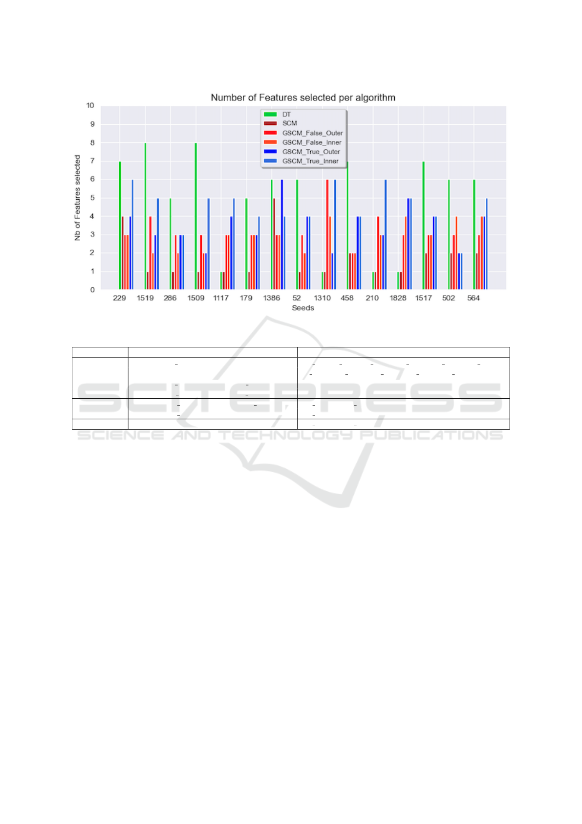
Figure 1: Number of feature return per algorithm at each seed (iteration).
Table 2: Features and Pathways selected by the best model of each algorithm type.
Algorithm Features Pathways
DT
uc002vwt.2 MLPH [G 455, G 1029, G 10245, G 11700, G 15952, G 25302,
G 30827, G 33710, G 44607, G 51709, G 52337]
SCM
uc002vwt.2 MLPH, uc002hul.3 RARA,
uc009wsd.2 HDGF, uc001jpo.1 TSPAN15 Not Shown (too much values)
GroupSCM
cg17095936 TBX19, cg10305797 KRTDAP, [G 82372], [G 82372],
cg18267381 ZNF385D [G 82372]
GroupSCM* hsa-mir-18a, hsa-mir-190b [G 80747], [G 81521]
group case), if the model selects some rules outside
the same pathways the conclusion is that the correct
explanation (from the experiment) is inter-groups re-
lated (since the rules belong to different pathways). In
the second case (the outer-group case), if the model
selects rules from the same pathways (i.e. it uses the
priors) meaning that the correct explanation is intra-
groups related. But overall, looking at the results in
table 1, the metric scores are not different from in-
ner versus outer update for the GroupSCM. Even if
it is for different c values. Despite being a little bit
less performing than the SCM, the GroupSCM pro-
duce sparser rules: three rules selected versus five
rules selected for the SCM. This comparison is on
the dataset with all the features. The results are even
sparser when considering the experiment with just the
features belonging to a known pathway. This situation
selects two rules. The sparser model implies easier in
vivo experimentation and validation.
Interestingly, the SCM selects almost all rules in
the RNA omics components and the GroupSCM se-
lect the rules either in the CpGs omics part or the
miRNA part (table 2). The main observation here
is while both the DT and the SCM seem to select
only RNA isoforms rules therefore the RNA omics
views only, the GroupSCM overlooks this view to se-
lect rules from either the CpGs (methylome view) or
the miRNA (miRNA views). This is useful finding
since CpGs and miRNA impact the translation there-
fore the gene expressions levels. Biologically speak-
ing, the algorithm is putting greater emphasis on the
upstream of the biology principal theory. Let’s recall
here one of the hidden goals is to see how well in-
vestigating all the omics together would perform on
the prediction task of determining the TNBC vs. non-
TNBC patients. In that case, the algorithm still con-
centrates on just one component of the omics view
but in a more integrative fashion. Indeed knowing if
the CpGs sites are hyper or under methylated is also
informative on the genes expression level, since we
have the pathways of the genes, those sites regulate.
It is a similar process for the miRNA. Their levels of
expression (over or under) also affect the gene expres-
sions level, and knowing their pathways, we can see
the downstream impact of the miRNAs on gene ex-
pressions. The GroupSCM enables a bigger picture
BIOINFORMATICS 2021 - 12th International Conference on Bioinformatics Models, Methods and Algorithms
78
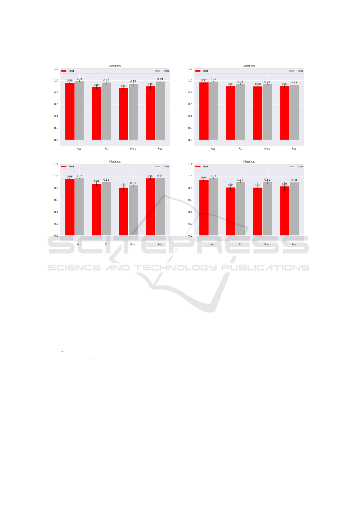
(a) Decision Tree (b) SCM
(c) GroupSCM on the complete dataset (d) GroupSCM on the dataset without the features non-belonging to a pathway
Figure 2: DT-SCM-GroupSCM Mean Metrics Results (Accuracy, F1-score, Precision and Recall)(Train (Gray) Test (Red)).
and observation of the biomarker discovery process
in a more global way.
We elect to analyze the features returned by
the GroupSCM in the experiment without the fea-
tures not belonging to a pathway. The model ob-
tains from this experimentation is a two-rule con-
junction: hsa-mir-18a and hsa-mir-190b. Accord-
ing to (Weizmann, 2020a) diseases associated with
mir18A include thyroid gland anaplastic carcinoma
and medulloblastoma. Among its related pathways
are Parkinson’s disease pathway and DNA damage
response. In our database: mir18A belongs to path-
way G 80747 in our experimentation (http://mirdb.
org/cgi-bin/mature mir.cgi?name=hsa-miR-18a-3p).
This biomarker is known to heavily impact numer-
ous pathways or interactions in many cancers. (Ko-
matsu et al., 2014) described mir18A as an impor-
tant biomarker in cancer since mir18A, which is lo-
cated in the potentially oncogenic miR-17-92 clus-
ter, is a highly expressed microRNAs in several
types of cancers. (Li et al., 2016) demonstrated
that tamoxifen resistance in breast cancer cells is en-
hanced through a miR-18a-HIF1 feedback regulatory
loop. Recently, (Zhang et al., 2019) also showed
that SREBP1, targeted by miR-18a-5p, modulates
epithelial-mesenchymal transition in breast cancer
via forming a co-repressor complex with Snail and
HDAC1/2. This literature review confirms that our
algorithm targets an already known biomarker in can-
cer studies. But there is no link specifically to the
TNBC phenotype. According to (Weizmann, 2020b),
there are no diseases linked to mir190B. Nevertheless,
(Cizeron-Clairac et al., 2015) proved that mir190B is
the highest up-regulated miRNA in ER-positive com-
pared to ER-negative breast tumors. Making it a po-
tential new biomarker for the triple-negative breast
cancer. (Zhao et al., 2020) recently demonstrated that
long non-coding RNA TUSC8 inhibits breast cancer
growth and metastasis via miR190b-5p/MYLIP axis.
These evidences show the ability of our model to dis-
cover biomarkers for the TNBC prediction problem.
As we can see for both of these miRNAs there is no
direct connection between them and the TNBC phe-
notype but our study suggests otherwise. The next
step will be to analyze those biomarkers in in vivo set-
tings to have solid confirmation of the discovery. We
proceeded with a statistical analysis of the biomark-
ers retrieved and analyzed the expression level in the
population with the classical t-test and the p-values.
In figure 3 we plotted the expression levels of both
Applying PySCMGroup to Breast Cancer Biomarkers Discovery
79
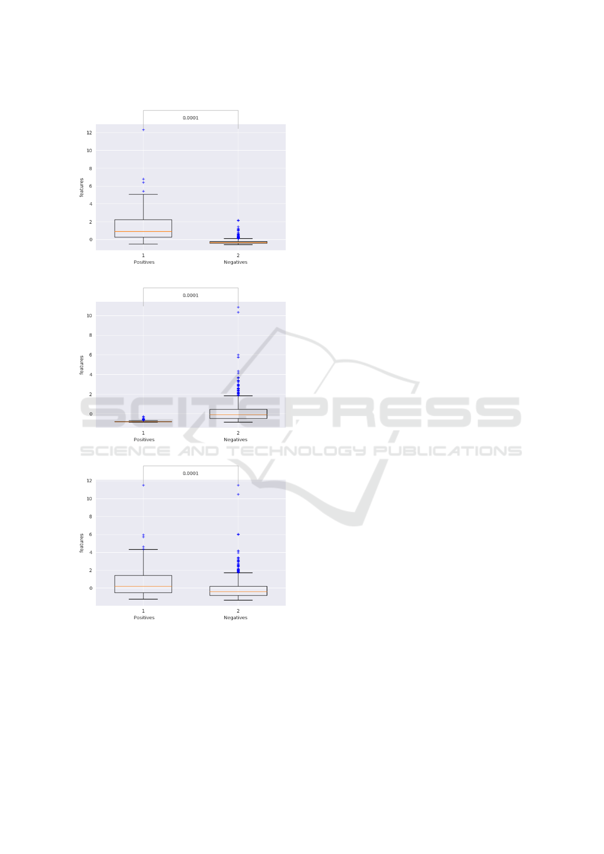
(a) hsa-mir-18a
(b) hsa-mir-190b
(c) hsa-mir-18a & hsa-mir-190b
Figure 3: Expression levels of the hsa-mir-18a (a), hsa-mir-
190b (b) and both (c) in the TNBC vs non-TNBC.
features independently alone (fig 3 a & b) and to-
gether. The conclusion is both of them are statisti-
cally significant with hsa-mir-18a more expressed in
the TNBC and hsa-mir-190b in the non-TNBC. To-
gether they are substantially expressed in the TNBC
examples improving the significance.
5 CONCLUSION
We present and apply an extension of the SCM to
an algorithm using a prior on the pathways of appar-
tenance of the features. In this particular case, the
algorithm yields interesting results biomarkers while
maintaining a good statistical scores overall. This al-
gorithm is a good addition to the precision medicine
field using the pathway interaction to find the appro-
priate biomarkers related to a specific disease. It is
sparse and interpretable which suits clinician expec-
tations. Despite the findings, additional in vivo exper-
imentations should be completed continuing the im-
provements of the model performance of data-driven
predictions and to provide validated evidence linking
specific biomarkers to a disease phenotype.
COMPETING INTERESTS
The authors declare that they have no competing in-
terests.
AUTHOR’S CONTRIBUTIONS
OMA designed the algorithm and the experimentation
and wrote this article. PT co-designed the algorithm.
JC and FL supervised the work and contributed to the
redaction of the manuscript.
ACKNOWLEDGEMENTS
A special thanks to Emmanuel Noutahi for his inputs
in this work. The work was supported by the Canada
Research Chair in Medical genomics (JC), Compute
Canada, Institute Intelligence and Data (IID) and
Centre de recherche en donn
´
ees massives (CRDM).
REFERENCES
Bareche, Y., Venet, D., Ignatiadis, M., Aftimos, P., Piccart,
M., Rothe, F., and Sotiriou, C. (2018). Unravelling
triple-negative breast cancer molecular heterogeneity
using an integrative multiomic analysis. Annals of On-
cology, 29(4):895–902.
Cizeron-Clairac, G., Lallemand, F., Vacher, S., Lidereau,
R., Bieche, I., and Callens, C. (2015). Mir-190b,
the highest up-regulated mirna in erα-positive com-
pared to erα-negative breast tumors, a new biomarker
in breast cancers? BMC cancer, 15(1):499.
BIOINFORMATICS 2021 - 12th International Conference on Bioinformatics Models, Methods and Algorithms
80

Delogu, F., Kunath, B., Evans, P., Arntzen, M., Hvid-
sten, T., and Pope, P. (2020). Integration of abso-
lute multi-omics reveals dynamic protein-to-rna ratios
and metabolic interplay within mixed-domain micro-
biomes. Nature Communications, 11(1):1–12.
Dinu, I., Potter, J. D., Mueller, T., Liu, Q., Adewale, A. J.,
Jhangri, G. S., Einecke, G., Famulski, K. S., Halloran,
P., and Yasui, Y. (2007). Improving gene set analysis
of microarray data by sam-gs. BMC bioinformatics,
8(1):242.
Doshi-Velez, F. and Kim, B. (2017). Towards a rigorous sci-
ence of interpretable machine learning. arXiv preprint
arXiv:1702.08608.
Drouin, A., Gigu
`
ere, S., D
´
eraspe, M., Marchand, M., Tyers,
M., Loo, V. G., Bourgault, A.-M., Laviolette, F., and
Corbeil, J. (2016). Predictive computational pheno-
typing and biomarker discovery using reference-free
genome comparisons. BMC genomics, 17(1):1–15.
Freedman, M. L., Monteiro, A. N., Gayther, S. A., Coet-
zee, G. A., Risch, A., Plass, C., Casey, G., De Biasi,
M., Carlson, C., Duggan, D., et al. (2011). Principles
for the post-gwas functional characterization of cancer
risk loci. Nature genetics, 43(6):513–518.
G
¨
unther, O. P., Chen, V., Freue, G. C., Balshaw, R. F.,
Tebbutt, S. J., Hollander, Z., Takhar, M., McMaster,
W. R., McManus, B. M., Keown, P. A., et al. (2012). A
computational pipeline for the development of multi-
marker bio-signature panels and ensemble classifiers.
BMC bioinformatics, 13(1):326.
Heuschkel, M. A., Skenteris, N. T., Hutcheson, J. D.,
van der Valk, D. D., Bremer, J., Goody, P., Hjortnaes,
J., Jansen, F., Bouten, C. V., van den Bogaerdt, A.,
et al. (2020). Integrative multi-omics analysis in cal-
cific aortic valve disease reveals a link to the formation
of amyloid-like deposits. Cells, 9(10):2164.
Iorio, M. V., Ferracin, M., Liu, C.-G., Veronese, A., Spizzo,
R., Sabbioni, S., Magri, E., Pedriali, M., Fabbri, M.,
Campiglio, M., et al. (2005). Microrna gene expres-
sion deregulation in human breast cancer. Cancer re-
search, 65(16):7065–7070.
Karczewski, K. J. and Snyder, M. P. (2018). Integrative
omics for health and disease. Nature Reviews Genet-
ics, 19(5):299.
Komatsu, S., Ichikawa, D., Takeshita, H., Morimura, R.,
Hirajima, S., Tsujiura, M., Kawaguchi, T., Miyamae,
M., Nagata, H., Konishi, H., et al. (2014). Circulat-
ing mir-18a: a sensitive cancer screening biomarker
in human cancer. in vivo, 28(3):293–297.
Lao, V. V. and Grady, W. M. (2011). Epigenetics and col-
orectal cancer. Nature reviews Gastroenterology &
hepatology, 8(12):686.
Lehmann, B. D., Bauer, J. A., Chen, X., Sanders, M. E.,
Chakravarthy, A. B., Shyr, Y., and Pietenpol, J. A.
(2011). Identification of human triple-negative breast
cancer subtypes and preclinical models for selection
of targeted therapies. The Journal of clinical investi-
gation, 121(7):2750–2767.
Li, X., Wu, Y., Liu, A., and Tang, X. (2016). Long
non-coding rna uca1 enhances tamoxifen resistance
in breast cancer cells through a mir-18a-hif1α feed-
back regulatory loop. Tumor Biology, 37(11):14733–
14743.
Liberzon, A., Subramanian, A., Pinchback, R., Thor-
valdsd
´
ottir, H., Tamayo, P., and Mesirov, J. P. (2011).
Molecular signatures database (msigdb) 3.0. Bioinfor-
matics, 27(12):1739–1740.
Liu, Y., Devescovi, V., Chen, S., and Nardini, C. (2013).
Multilevel omic data integration in cancer cell lines:
advanced annotation and emergent properties. BMC
systems biology, 7(1):14.
Marchand, M. and Shawe-Taylor, J. (2002). The set cover-
ing machine. Journal of Machine Learning Research,
3(Dec):723–746.
Miller, T. (2019). Explanation in artificial intelligence: In-
sights from the social sciences. Artificial Intelligence,
267:1–38.
Molnar, C. (2019). Interpretable Machine Learning. https:
//christophm.github.io/interpretable-ml-book/.
Rappoport, N., Safra, R., and Shamir, R. (2020). Monet:
Multi-omic module discovery by omic selection.
PLOS Computational Biology, 16(9):e1008182.
Ritchie, M. D., Holzinger, E. R., Li, R., Pendergrass, S. A.,
and Kim, D. (2015). Methods of integrating data to
uncover genotype-phenotype interactions. Nature re-
views. Genetics, 16(2):85.
Singh, A., Gautier, B., Shannon, C. P., Vacher, M., Rohart,
F., Tebutt, S. J., and Le Cao, K.-A. (2016). Diablo-
an integrative, multi-omics, multivariate method for
multi-group classification. bioRxiv, page 067611.
Stark, C., Breitkreutz, B.-J., Reguly, T., Boucher, L., Bre-
itkreutz, A., and Tyers, M. (2006). Biogrid: a general
repository for interaction datasets. Nucleic acids re-
search, 34(suppl 1):D535–D539.
Tian, S., Wang, C., and Wang, B. (2019). Incorporating
pathway information into feature selection towards
better performed gene signatures. BioMed research
international, 2019.
Weigelt, B., Baehner, F. L., and Reis-Filho, J. S. (2010).
The contribution of gene expression profiling to breast
cancer classification, prognostication and prediction:
a retrospective of the last decade. The Journal of
Pathology: A Journal of the Pathological Society of
Great Britain and Ireland, 220(2):263–280.
Weizmann, I. o. S. (2020a). Mir18a. https://www.
genecards.org/cgi-bin/carddisp.pl?gene=MIR18A.
Accessed: 2020-10-21.
Weizmann, I. o. S. (2020b). Mir190b. https://www.
genecards.org/cgi-bin/carddisp.pl?gene=MIR190B.
Accessed: 2020-10-21.
Wu, D., Lim, E., Vaillant, F., Asselin-Labat, M.-L., Vis-
vader, J. E., and Smyth, G. K. (2010). Roast: ro-
tation gene set tests for complex microarray experi-
ments. Bioinformatics, 26(17):2176–2182.
Yuan, Y., Liu, L., Chen, H., Wang, Y., Xu, Y., Mao, H., Li,
J., Mills, G. B., Shu, Y., Li, L., et al. (2016). Com-
prehensive characterization of molecular differences
in cancer between male and female patients. Cancer
cell, 29(5):711–722.
Zhang, N., Zhang, H., Liu, Y., Su, P., Zhang, J., Wang, X.,
Sun, M., Chen, B., Zhao, W., Wang, L., et al. (2019).
Applying PySCMGroup to Breast Cancer Biomarkers Discovery
81

Srebp1, targeted by mir-18a-5p, modulates epithelial-
mesenchymal transition in breast cancer via forming
a co-repressor complex with snail and hdac1/2. Cell
Death & Differentiation, 26(5):843–859.
Zhao, L., Zhou, Y., Zhao, Y., Li, Q., Zhou, J., and Mao,
Y. (2020). Long non-coding rna tusc8 inhibits breast
cancer growth and metastasis via mir-190b-5p/mylip
axis. Aging (Albany NY), 12(3):2974.
BIOINFORMATICS 2021 - 12th International Conference on Bioinformatics Models, Methods and Algorithms
82
