Contrast Ratio during Visualization of Subsurface Optical

Inhomogeneities in Turbid Tissues: Perturbation Analysis

Gennadi Saiko

and Alexandre Douplik

Department of Physics, Ryerson University, Toronto, Canada

Keywords: Biomedical Imaging, Diffuse Approximation, Turbid Tissues.

Abstract: Visualization and monitoring of the capillary loops and microvasculature patterns in dermis and mucosa are

of interest for various clinical applications, including early cancer and shock detection. We developed an

approach for the assessment of the contrast ratio during the visualization of subsurface optical heterogeneities.

Using the diffuse approximation and perturbation analysis, we considered light absorption heterogeneities as

negative light sources. We estimated the contrast ratio as a function of the surface layer's optical properties

for diffuse and collimated wide beam illumination. Based on findings, we formulated several practical

suggestions: a) proper selection of camera (with maximum dynamic range) is of paramount importance, b)

narrow-band illumination is more efficient than white light illumination, and c) use of collimated light

provides up to 60% improvement in contrast vs. diffuse illumination. Obtained results can be used for the

optimization of imaging techniques

1 INTRODUCTION

Visualization and monitoring of capillary loops in the

dermis and mucosa are of interest for various clinical

applications, including early cancer and shock

detection (Kanawade, 2010). Unusual capillary and

capillary loop shapes can be precursors of cancer

transformations (e.g., angiogenesis) or auto-immune

diseases (scleroderma). Rapid changes in their shape

and sizes can be one of the first signs of shock

development. This interest drives continuous

improvements in image quality in traditional optical

systems and rapidly emerging lensless (Schelkanova,

2016) optical systems.

Because of the low-contrast nature of images of

absorption patterns ("defects") in highly-light-

scattering biotissues, several techniques were

proposed to increase this contrast – (1) a narrow band

imaging providing a better contrast than white light

imaging (Saiko, 2020); (2) optical clearing to

improve the imaging quality; (3) transformation and

analysis of the image into a different colorspace (e.g.,

RGB->HSV) where subsurface inhomogeneity or

"defect" appears enhanced (Zhanwu, 2006). In

particular, Goffredo et al. (Goffredo, 2012)

https://orcid.org/0000-0002-5697-7609

https://orcid.org/0000-0001-9948-9472

considered various color channel transformations to

increase sensitivity and specificity for such defect

discovery.

Given the continuous efforts to increase the

superficial tissue image quality, it is essential to

estimate its potential limitations. In our previous

works, we have tried to evaluate the limits of defect

detectability; namely a defect detectability depth (a

maximum depth at which the defect can be detected)

using computer simulations and a simple lattice

model (Saiko, 2012). Initial assessment predicted

(Saiko, 2012) that the detectability depth is limited by

1/ '



, where



is the reduced scattering

coefficient of the surface layer. However, more

rigorous analysis is required, which needs to include

quantifiable parameters relevant, in particular, to

human perception. A contrast ratio defined according

to Weber's law as

 



cx I Ix I

, where I

and I(x) is the intensity at the background and a point

x, respectively, can serve as such parameter (Saiko,

2014a; Saiko, 2020)). We define a threshold contrast

ratio, c

th,

as a minimum contrast ratio, which can be

resolved by a particular optical device. Our definition

implies that an optical system can not visualize the

Saiko, G. and Douplik, A.

Contrast Ratio during Visualization of Subsurface Optical Inhomogeneities in Turbid Tissues: Perturbation Analysis.

DOI: 10.5220/0010374100940102

In Proceedings of the 14th International Joint Conference on Biomedical Engineering Systems and Technologies (BIOSTEC 2021) - Volume 2: BIOIMAGING, pages 94-102

ISBN: 978-989-758-490-9

defect if the measured contrast ratio is less than c

Respectively, a detectability depth Z can be defined

as a defect depth, where the measured contrast ratio

for the defect is equal to c

. Z is a function of a) the

threshold contrast ratio, b) the optical tissue

parameters (absorption coefficient, scattering

coefficient, index of refraction, anisotropy factor),

and c) defect parameters (volume, incremental

absorption coefficient, and depth). Even though for a

human eye, the threshold contrast ratio is around

0.1(Le, 2013), images with lower contrast ratio can be

digitally enhanced and still can be used for feature

examination or pattern recognition.

In automated processing scenarios, the threshold

contrast ratio is limited by the camera's dynamic

range, and we can estimate the threshold contrast

ratio, which can be obtained using commercially

available cameras. In the most typical scenario (e.g.,

with USB2 cameras), commercial cameras use 24bits

for each pixel (3 colors x 8bits). A standard camera

has 10-bit analog-to-digital converter (ADC), and due

to bandwidth restriction in USB2 format, just 8 bits

are employed. Thus, each channel's dynamic range is

=256, making the camera facilitate the contrast

ratio up to

_max

0.004

c 



. A more realistic

dynamic range (40%-80% of maximum) gives

=0.005-0.01. Similarly, for more advanced

cameras (e.g., USB3 or GigE), each color channel is

represented by 10-12bits, and the real dynamic range

can be as high as 1600-3200, which consequently

translates into c

=0.0003-0.0006. In our assessments

below, we will use c

=0.01 and 0.001 as threshold

contrast ratios, representing cameras with 8 and 12

bits per channel.

An analytical dependence of the contrast ratio on

the depth of inhomogeneity location has been found

(Dolin, 1997) for refractive index-matched boundary.

In (Aksel, 2011), an absorber's depth was assessed

using spatially resolved diffuse reflectance

measurements. In the current work, we will evaluate

how the depth of inhomogeneity location and optical

parameters of the surrounding biotissue affect the

image contrast in realistic conditions: a) refractive

index mismatched boundary, and b) clinically

relevant illumination scenarios (collimated and

diffuse wide beam illumination). We will then use

this information to find the detectability depth for

such a defect for a particular optical system, which we

will characterize using the threshold contrast ratio.

In a nutshell, we will determine the contrast ratio

for a particular defect (defects), characterized by

volume V and absorption coefficient



, and located

at the depth Z inside the tissue. Finding an exact

solution to this problem in the general case is

problematic. We will be looking for an approximate

solution. For this purpose, we have developed a

perturbation approach focusing on two typical

illumination scenarios in biotissue imaging and

spectroscopy (Saiko, 2014b): diffuse illumination

(e.g., ambient light) and collimated wide beam

illumination. To quantify the relative impact of each

optical parameter on the detectability depth Z, we will

determine dimensionless sensitivities (the relative

change in the detectability depth Z for a given relative

change in a parameter p, (



Z/Z)/(



p/p)) for all

parameters (scattering or absorption coefficient,

index of refraction, etc.).

2 METHODS

2.1 Tissue Model

Human skin and mucosal tissues have a layered

structure (Meglinski, 2002). Based on our primary

task to visualize the capillary grid, we can group

covering tissues into (I) bloodless epithelium, (II)

blood-containing papillary layer of the dermis (skin),

or lamina propria (mucosa), and (III) underlying

tissues (see Fig 1A). Living cells in epithelium

receive oxygen and nutrients through the diffusion

from capillaries located in the papillary layer

underneath. Thus, the thickness of living cells

epithelium layers is limited by the oxygen diffusion

length and typically does not exceed 100m.

However, the stratum corneum, which includes "non-

supplied" cells, can be much thicker in some organs,

such as feet, soles, or palms.

2.2 Geometry

Based on our tissue model, the epithelium (including

stratum corneum) can be considered an optical filter

that covers absorption features and deteriorates the

image's quality. To evaluate how the measured

contrast ratio is affected by the presence of this

outermost layer, we can consider the following model

(see Fig 1B): the homogeneous top layer (Layer I)

covers Layer II, which consists of 2 areas: a)

homogeneous background, b) capillaries, which can

be considered as heterogeneous (either absorption or

scattering) features or "defects." Below this layer II,

there is another layer III, which represents all

underlying tissues. As we are interested in estimating

the effects of the outermost surface layer, in order to

simplify calculations, we can consider simplified

geometry (Fig 1C): the homogeneous semi-infinite

Contrast Ratio during Visualization of Subsurface Optical Inhomogeneities in Turbid Tissues: Perturbation Analysis

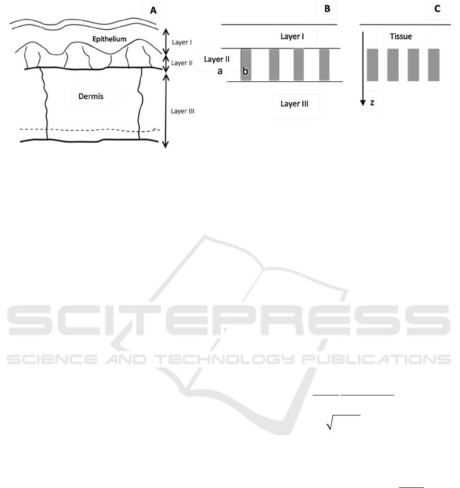
Figure 1: The logical transition from tissue microstructure (A) to heterogeneous dermis layer representation (B) to geometry

that allows evaluating upper bound on the contrast ratio (C). Areas (a) and (b) of the panel B are background tissue and

capillary (defect), respectively.

tissue characterized by an absorption coefficient



and "defects" described by the volume V and

absorption coefficient





and located at the

depth Z (here



is an incremental absorption

coefficient associated with the defect). In this case,

the contrast presented by the features will be

maximized, and we can estimate the upper bound (the

best-case scenario) for visualization of these

particular features.

2.3 Mathematical Model

The light propagation problem in homogeneous tissue

can be solved exactly for specific geometries (e.g.,

slab, semi-space, or spheroid in diffuse

approximation, slab and semi-space in Kubelka-

Munk model (see, e.g. (Saiko, 2014b)). The presence

of an arbitrary defect complicates things significantly,

and we have to look for an approximate solution. A

perturbation theory can be a useful approach to find

such an approximate solution: we start from the exact

solution for the semi-space geometry and add the

defect as a perturbation. Our perturbation approach

consists of the following steps:

1. We find a solution for light distribution in

homogeneous semi-infinite tissue (the radiant energy

fluence rate

()r





(W/m

)).

2. If we know the radiant energy fluence rate

()r





at some particular point



, then we can

calculate additional (or incremental) absorbed optical

power density

()

 



(W/m

) for some optical

heterogeneity with the absorption coefficient





located at this point. If the volume of the

heterogeneity is V, then the additional power

absorbed at this heterogeneity will be

()

 



(W).

3. Alternatively, the heterogeneity can be

considered a negative (or inverse) point source with

power

()









, located at the point



. The

radiant energy fluence rate induced by such a source

can be calculated exactly.

This problem can be analyzed using the diffuse

approximation (Star, 2011).

Step 1: For a semi-infinite medium with wide

beam diffuse illumination, the total radiant energy

fluence rate within the tissue far from the borders of

the beam depends only on the depth z (Eq. 6.88 in

(Star, 2012)):

exp( )

()

eff













(1)

Where

eff a





1/3





(1 )

tr a s



 

, r

is the coefficient of

reflection of diffuse light on the border of tissue and

air (r

can be approximated using the relative index

of refraction n: r

≈1-n

-2







. Here

without losing generality (we are looking for the

contrast ratio, which is dimensionless), we also

assumed that the incident light's surface density is 1

(W/m2).

Similarly, we can solve the semi-infinite problem

for wide beam collimated illumination. The

difference here is the presence of collimated term,

which dissipates proportionally to

exp( ( ) )





. For the biologically relevant

BIOIMAGING 2021 - 8th International Conference on Bioimaging

case,





we have an expression (Eq. 6.83 in

(Star, 2012)):

exp( )

()

2exp( ( ) )

eff















(2)

The advantage of the wide beam diffuse

illumination scenario is that it allows obtaining

closed-form expressions. We omit collimated light

calculations for the sake of brevity and present only

results.

Step 2: The additional power absorbed at the

inhomogeneity can be found by multiplication of

Eq.1 or 2 on V



Step 3: The diffuse source with power P in

isotropic medium generates radiant energy fluence

rate on the distance R from the source

() exp( )

seff









(3)

Thus, we can represent our defect as the point

source described by Eq.3, where power P is the power

calculated on step 2 with a minus sign (negative

source). To take into account the boundary

conditions, we can use the diffusion dipole model

(Frerrerd, 1973; Kienle, 1994). In addition to the

initial source located at depth Z, we can consider the

second source (with opposite sign) located on the

distance 2h+Z above the surface. In this case, total

flux approximately satisfies realistic boundary

condition for all r (

rxy

) and z=0

(Haskell, 1994)

(, )

(, ) 0

rz h









(4)

3 RESULTS

If the inhomogeneity is located at (0,0,Z), then the

fluence rate at any point on the surface of the tissue

surface (here we assume cylindrical coordinates) in

the presence of mismatched border will be:

221/2

3()

()

exp( ( ) )

()

exp( ((2 ) ) )

((2 ) )

atr

eff

hZ r

  





































(5)

Where



(Z)=



(Z) for diffuse illumination (Eq.1)

and



(Z)=



(Z) for collimated illumination (Eq.2).

Another realistic clinical scenario is to resolve

two heterogeneities located under the surface using

imaging techniques. It can be the case for assessing

whether an imaging technique can visualize each

blood capillary separately. Thus, we will consider two

geometries: a single defect or heterogeneity (Fig. 2A)

and two identical defects on the same depth (Fig. 2B).

Figure 2: Geometry of heterogeneities: a single defect (A)

and two defects (B).

3.1 Contrast in Case of a Single

Heterogeneity

Let's consider a single inhomogeneity located at

(0,0,Z) (see Fig 2A). Far from the inhomogeneity, its

effect is negligible. Thus, we can take the unperturbed

flux rate on the surface at this point as a background

(



(0)). Near the inhomogeneity, we cannot ignore

the flux rate from the inhomogeneity,



(r). If we

compare the background flux with the fluence rate on

the surface in the presence of the inhomogeneity

(



(r)=



(0)+



(r)), we can calculate the contrast ratio

at any point on the surface of the tissue

() ()

()

(0)

 







(6)

here again



(0)=



(0) for diffuse illumination (Eq.1)

and



(0)=



(0) for collimated illumination (Eq.2).

3.1.1 Diffuse Illumination

For diffuse illumination from Eq.5 with



(Z)=



(Z)

and Eq.6, we will get:

221/2

3exp()

()

exp( ( ) )

()

exp( ((2 ) ) )

((2 ) )

tr a eff

eff

hZ r

 



































(7)

Immediately above the heterogeneity (r=0) from

Eq.7, we can get a compact expression

Contrast Ratio during Visualization of Subsurface Optical Inhomogeneities in Turbid Tissues: Perturbation Analysis

Figure 3: Panel A- radial dependence of the contrast ratio (collimated illumination- left side, diffuse illumination –right side)

on the surface above the defect located at depth 0.05mm (solid red line), 0.1mm (dotted blue line) and 0.2mm (dashed green

line). Panel B- the contrast in the point above the defect c(0) as a function of the defect depth (in mm) for wide beam diffuse

(solid red line) and collimated (dotted blue line) illumination. Panel C- the ratio of contrasts for collimated illumination and

diffuse illumination. Tissue parameters were:



=0.033mm

-1

and



=5mm

-1

(reticular dermis),



=28mm

-1

(the whole blood

with 70% oxygenation at 532nm), V=20x20x20m

, n=1.33.

3exp(2)

(0)

exp( 2 )

tr a eff

eff

ZhZ



 





















(8)

3.1.2 Collimated Illumination

We can also analyze how the contrast will be different

for the same defect for diffuse and collimated

illumination. As we just discussed, the contrast at any

point on the surface of the tissue for the defect located

on the depth Z taking into account Eq.6 would be

() ()/ (0)

cr r





, here

(z)



is the

unperturbed flux distribution for either diffuse light

(Eq.1) or collimated light (Eq.2). Thus, taking into

account that for our negative source



(r)~-





Z)~



Z) after simple reducing, we can find

that the ratio of contrasts for collimated light and

diffuse light will be

()/ (0)

exp( ( ) )

aseff













(9)

here for the sake of brevity, we introduced

eff









We have analyzed the problem in a realistic case

of the upper part of the capillary loop in the

dermis:



=0.033mm

-1

and



=5mm

-1

for reticular

dermis (Meglinski, 2002),



=28mm

-1

(the whole

blood with 70% oxygenation at 532nm),

V=20x20x20m

, n=1.33. Results are presented in

Fig 3.

Fig 3B shows that such defects can be visualized

(with c

=0.001) till approximately 0.07 mm for

diffuse illumination and 0.09 mm for collimated

illumination.

3.2 Contrast in Case of Double

Heterogeneity

To analyze this problem for diffuse illumination, let's

consider two heterogeneities located at (X,0,Z) and (-

X,0,Z) (see Fig 2B). If we compare fluence rate on the

surface far from the heterogeneities (background,



(0)) and the fluence rate on the surface in the

presence of the inhomogeneities (



(x,y)=



(0)



(x,y)) we can calculate contrast ratio at any point

(x,y,0) on the surface of the tissue. Using Eq. 5 for

each inhomogeneity, we can get Eq. 10.

To distinguish these two heterogeneities, there

should be some contrast between a point above any of

these heterogeneities (e.g. (X,0,0)) and the point

between two heterogeneities (0,0,0)- see Eq.11

So, if



c>c

, then we can distinguish two

heterogeneities. In the opposite case, we will see them

as a single heterogeneity with the length 2X.

BIOIMAGING 2021 - 8th International Conference on Bioimaging

(10)

221/2 221/2

221/2

3 exp( ) exp( )

(,0) (0,0)

exp( ( 4 ) ) exp( (2 )) exp( ((2 ) 4 ) )

(4) 2 ((2)4)

exp( ( ) ) exp( ((2

()

tr a eff eff

eff eff eff

eff eff

VZ Z

ccX c

Z X hZ hZ X

ZX h

  











    





   

 



 





221/2

)))

((2 ) )

hZ X













(11)

We have analyzed the problem in a realistic case

of upper part of capillary loop in dermis:



=0.033mm

-1

and



=5mm

-1



=28mm

-1

V=20x20x20m

, n=1.33, X=0.1mm. Results are

presented in Fig 4.

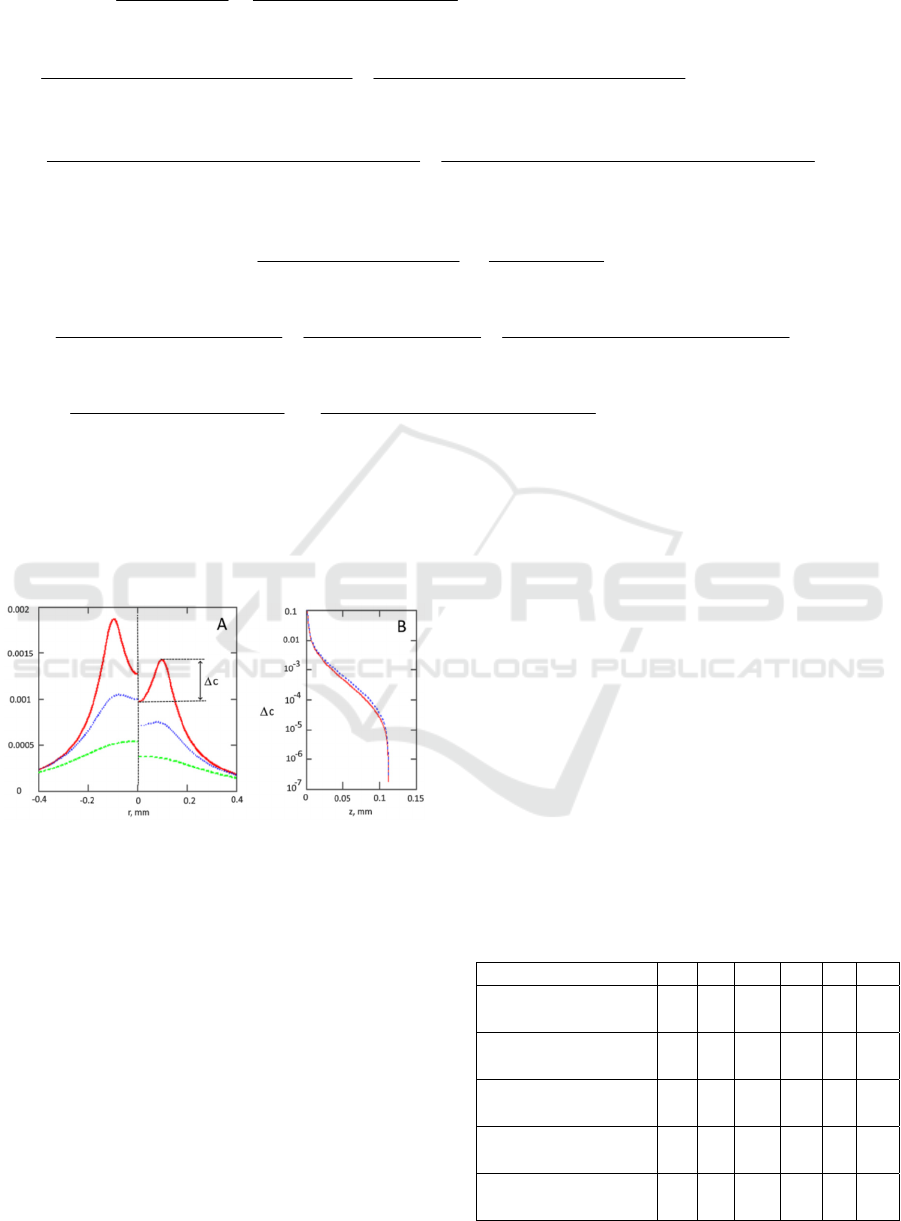
Figure 4: Panel A- Dependence of the contrast ratio

(collimated illumination – left side, diffuse illumination-

right side) on the surface above the defects located at depth

0.05mm (solid red line), 0.1mm (dotted blue line) and

0.2mm (dashed green line). Panel B- c(difference in

contrast in the point above the defect c(X,0) and between

defects c(0,0)) as a function of the defect depth Z (in mm)

for wide beam diffuse (solid red line) and collimated

(dotted blue line) illumination. Tissue parameters:



=0.033mm

-1



=5mm

-1



=28mm

-1

(the whole blood

with 70% oxygenation at 532nm), V=20x20x20m

n=1.33. Half distance between defects X=0.1mm.

Resolution depth for such scenario is

approximately 0.034mm (for c

=0.001).

In addition, we have calculated the sensitivity of

observables (detectability depth and contrast ratio) to

changes in any optical tissue parameters (z/z/p/p,

where p is an optical tissue parameter, e.g., absorption

coefficient) by varying each optical parameter (





,V, n) and half-distance between defects X by -

20%, -10%, 10%, and 20%. We also split



into



and g and studied each of these variables separately

(assuming g=0.8,



=25mm

-1

). Results for the normal

skin (Meglinski, 2002) are presented in Table 1.

For example, one can see that in the case of a

single defect imaged with an 8-bit camera (c

=0.01),

the largest relative impact has the anisotropy factor:

1% change in the anisotropy factor leads to a 3.6%

change in the detectability depth. In this case, the

effect can be ranked (from the highest to the lowest):

the anisotropy factor, defect parameters (



, V),

scattering coefficient, index of refraction. The impact

of the absorption coefficient of the tissue is relatively

minimal.

Table 1: Dimensionless sensitivities ((z/z)/(p/p)) of

observables (in rows) to changes in optical parameters of

the tissue (



, g, n) and defect (



,V, X).

Observables 



g n X 

Detectability depth z for

=0.01 (single defect)

0.00 0.90 -3.60 0.10 n/a 0.90

Detectability depth z for

=0.001 (single defect)

-0.06 0.51 -2.15 0.41 n/a 0.72

Detectability depth z for

=0.01 (double defect)

0.00 0.79 -2.89 0.00 0.26 0.79

Detectability depth z for

=0.001 (double defect)

0.00 0.32 -1.43 0.00 0.67 2.59

Contrast ratio c for the

defect located at z=0.1mm

-0.06 0.76 -3.25 0.76 n/a 1.08

2 2 21/2 2 2 21/2

2221/2

3 exp( )

(, )

exp( ( ( ) ) ) exp( ( ( ) ) )

(( ) ) (( ) )

exp( ((2 ) ( ) ) ) exp(

((2 ) ( ) )

tr a eff

eff eff

cxy

ZxXy ZxXy

hZ xX y



 









 



 





   





 



 

2221/2

((2 ) ( ) ) )

((2 ) ( ) )

hZ xX y



 



 





Contrast Ratio during Visualization of Subsurface Optical Inhomogeneities in Turbid Tissues: Perturbation Analysis

4 DISCUSSION AND

CONCLUSIONS

We have analyzed several scenarios that can be used

for image quality characterization in tissue imaging.

We found that various optical parameters contribute

differently to the contrast ratio. The absorption

coefficient of the tissue does have a very minimal

impact. The most substantial effect has the anisotropy

factor g (due to our initial value g=0.8, it is

approximately four times (g/(1-g)) stronger than



followed by properties of the defect and scattering

coefficient of the tissue. The refraction index and the

distance between defects have minimal impact. These

data provide the relative impact of various factors on

the experiment's accuracy and can be used to guide

experimental and Monte Carlo simulations.

While a few tissue optical parameters can be

varied in an experiment (e.g., tissue scattering

coefficient and refraction index through optical

clearing), the absorption coefficient for

inhomogeneity is the single factor that can be varied

in practice. Moreover, the contrast linearly depends

on this factor, and detection depth strongly depends

on it as well (high sensitivity, see Table 1). Thus,

proper wavelength selection (e.g., at the absorption

peak of hemoglobin) is of paramount importance for

visualization.

We considered two realistic illumination

scenarios: wide beam diffuse illumination (e.g.,

ambient light) and wide beam collimated illumination

(e.g., a medical light source, laser). Results are very

similar. However, it should be noted that collimated

illumination provides better image contrast (see Fig

3B and 4B for comparison). For our parameters, 40%

contrast improvement can be achieved using

collimated illumination (see Fig 3C). We can estimate

the maximum enhancement provided by the

collimated light. Taking into account that

aeff







and using Eq.9, we can find that for

deep defects (





)

21 21

25 2(1 )(1 )

eff

arrh









(12)

In case of the matched boundary (

0r 

/5/(34/3)

cd a tr





(13)

Such as in most tissues



this ratio can be

estimated as 5/3. That means that for the matched

boundary, collimated light provides 66%

improvement over diffuse light. These results are in

agreement with previously reported models (Saiko,

2020).

If we know the contrast ratio associated with the

defect, we can assess whether a particular imaging

system can visualize it. Namely, if the camera's

threshold contrast ratio is above the defect contrast

ratio, the defect can be imaged. We assessed that the

realistic threshold contrast ratio for commercially

available cameras is in the 0.01-0.001 range for 8-12

bits cameras. Because the dynamic range of a camera

used in measurements is the primary factor limiting

the recognition of objects with low contrast, the

proper selection of a camera is vital for imaging

subsurface structures.

Out estimations of the defect detectability depth

are in a qualitative agreement with MC simulations

(Saiko, 2014a). In particular, MC simulations have

shown (Saiko, 2014a) that diffuse reflectance

spectroscopy can potentially identify absorption

inhomogeneities located at a depth of 0.5–1.0 of the

transport mean free path l

= 1/μ

It should be noted that the proposed "detectability

depth" is different from a mean sampling (or

interrogation) depth (see, e.g. (Bevilacqua, 2004)).

The mean sampling depth can be viewed as the first

moment of the photon scattering density function (or

PSDF) for various photon trajectories (e.g., in a

Monte Carlo simulation). The mean sampling depth

depends on the tissue's optical properties (



and'

)

and source-detector separation (if any). The

detectability depth depends on



and



, the

properties of the defect (namely volume V and

absorption coefficient



), and the imaging system's

properties (namely the threshold contrast ratio c

Conceptually, our approach is a perturbation

expansion. The zeroth term is the light distribution in

a homogeneous semi-infinite issue, and the first-order

term is the linear contribution caused by the presence

of inhomogeneities (defects).

To keep the perturbation approach valid, we need

to satisfy several conditions. Firstly, the light field

change within the defect caused by its absorption

properties should be small. Given that the defect in

our case is illuminated from all sides, then the impact

will be negligible if

1/3

/2 1





, which is satisfied

for our defect parameters.

Secondly, the diffuse approximation provides

accurate light distribution far from sources and

borders: when the mean optical free path (1/



) is

much smaller than the size under consideration. For

our quasi-1D problem, the defect depth z is the only

characteristic size and





. However, the diffuse

approximation is still a useful approximation, even

BIOIMAGING 2021 - 8th International Conference on Bioimaging

100

close to boundaries (Chai, 2008). In particular,

(Lehtikangas, 2012) found that the relative error of

fluence rate near the surface is between 3.73% and

6.31% for the DA when μ

= 50 mm

−1

and μ

= 5

−1

, respectively. Such as we intend to provide

rough estimations (e.g., feasibility assessment of

technology, estimate maximum detectability depth

for a particular wavelength, select appropriate bit

depth for the camera), we expect that its major

conclusions will hold.

In addition to general questions about the

applicability of the diffuse approximation, some

additional questions arise while using this

perturbation approach: a) what is the volume of the

heterogeneity to keep this approach valid, and b) if we

have multiple heterogeneities, what are the criteria to

make sure that they do not interact with each other,

namely that their impacts are additive.

To address the first question, we can consider that

we have a one-dimensional problem with constant

illumination in the horizontal plane in the zeroth

approximation. Thus, the defect will be small enough

if the light distribution within the defect will be

homogeneous:









, where l

is the vertical

size (the height on Fig 2A) of the defect. Taking into

account Eq.1, this condition can be rewritten as

eff z





The requirement (b) can be reformulated as

follows: the fluence rate induced by all other defects

is much smaller than the homogeneous field at this

point. Using Eq.1 and Eq.2, we can estimate the

required distance R between defects with volume V

as:

atr









, which is less than 1m for

our parameters.

In light of requirement (b), we can take a look at

the applicability of our approach to vertical (e.g.,

capillaries) and horizontal (e.g., nail fold capillaries)

linear heterogeneities. One can easily find that due to

slow descendants of the fluence rate induced by a

single defect (Eq.3), the integral of the fluence rate

diverges at any point of the continuous curve of

sources. Thus, even though it is possible to calculate

the impact of inhomogeneity in these scenarios, such

solutions' validity will be doubtful. Consequently,

this approach can be applied only to sets of discrete

heterogeneities with distances between them

atr







 

If the inhomogeneity's parameters are known

(e.g., in the case of a blood vessel), then the contrast

ratio can be used to extract the surface layer's

parameters, e.g., its thickness. Measuring contrast at

multiple wavelengths (e.g., multispectral or

hyperspectral imaging) may obtain further insights

into the epithelial layer's composition.

As a natural extension of previous works (Saiko,

2012, 2014a, 2014b), the current results explicitly

contain absorption coefficient, thus allowing a direct

MC verification.

In summary, we propose a simple perturbation

model, which links optical tissue parameters with the

contrast ratio in reflectance imaging geometry. Using

the proposed model, we derived explicit expressions

for the contrast ratio in the case of tissue imaging with

diffuse and collimated wide beam illumination. Using

the contrast ratio, the detectability depth can be

estimated for a particular imaging system. The

relative impact of optical tissue parameters on the

detectability depth can also be determined. The

proposed approach can be exploited for the

assessment and optimization of tissue imaging

techniques.

ACKNOWLEDGEMENTS

The authors would like to acknowledge the support

for this study from NSERC Discovery grant

(Douplik), Ryerson Health Fund, NSERC Engage

support, and infrastructural support from Institute for

Biomedical Engineering, Science and Technology

(IBEST), a partnership between Ryerson University

and St. Michael's Hospital (Toronto).

REFERENCES

Kanawade, R. et al., 2010, Vessel density modulation

detection in skin model by using spatially resolved

diffuse reflectance techniques for application of early

sign of shock detection. Photodiagnosis and

Photodynamic Therapy; 7: P14

Schelkanova, I. et al., 2016, Spatially resolved, diffuse

reflectance imaging for subsurface pattern visualization

toward development of a lensless imaging platform:

phantom experiments. J. Biomed. Opt.21 (1): 015004.

Saiko, G., Betlen, A., 2020, Optimization of Band Selection

in Multispectral and Narrow-Band Imaging: an

Analytical Approach, Adv. Exp Med Biol 1232:361-367.

Zhanwu, X., Miaoliang, Z., 2006, Color-based skin

detection: survey and evaluation. In: Proceedings of the

12th International Conference on Multi-Media

Modelling, vol 10, Beijing.

Goffredo, M. et al., 2012, Quantitative color analysis for

capillaroscopy image segmentation, Med Biol Eng

Comput 50:567–574

Contrast Ratio during Visualization of Subsurface Optical Inhomogeneities in Turbid Tissues: Perturbation Analysis

101

Saiko, G. Douplik, A., 2012, Real-Time optical monitoring

of capillary grid spatial pattern in epithelium by

spatially resolved diffuse reflectance probe, J Innov.

Opt. Heal. Scie., 05(02): 1250005

Saiko G. et al., 2014 Optical Detection of a Capillary Grid

Spatial Pattern in Epithelium by Spatially Resolved

Diffuse Reflectance Probe: Monte Carlo Verification,

Sel. Top. Quantum Electron. IEEE J. 20(2): 7000609

Le D. et al., 2013, Monte Carlo modeling of light–tissue

interactions in narrow band imaging, J. Biomed. Opt.,

18 (1): 010504-1–010504-3.

Dolin, L.S., 1997 On the possibility of detecting an

absorbing object in a strongly scattering medium using

the method of continuous optical sounding,

Radiophysics and Quantum Electr, 40(10): 799-812.

Aksel, E.B., et al., 2011, Localization of an absorber in a

turbid semi-infinite medium by spatially resolved

continuous-wave diffuse reflectance measurements. J

Biomed Opt.; 16(8):086010.

Saiko, G. Douplik, A., 2014, Reflectance of Biological

Turbid Tissues under Wide Area Illumination: Single

Backward Scattering Approach, Int. J. of Photoenergy,

241364

Meglinski, I. V. Matcher, S. J., 2002, Quantitative

assessment of skin layers absorption and skin

reflectance spectra simulation in the visible and near-

infrared spectral regions, Physiol. Meas. 23:741753.

Star, W.M., 2011, Diffusion Theory of Light Transport, in

Optical-Thermal Response of Laser-Irradiated Tissue

(2nd Ed) Ed. by A.J. Welch, Dordrech, NLD: Springer,

Frerrerd, R.J. Longini, R.L. 1973, Diffusion dipole source,

J. Opt. Soc. Am. 63: 336-337

Kienle, A., Patterson, M.S, 1994, Improved solutions of the

steady-state and the time-resolved diffusion equations

for reflectance from a semi-infinite turbid medium, J.

Opt. Soc. Am. A 14: 246-254.

Haskell R.C., et al., 1994, Boundary conditions for the

diffuse equation in radiative transfer, J. Opt. Soc. Am.

A 11: 2727-2741.

Bevilacqua F. et al., 2004, Sampling tissue volumes using

frequency-domain photon migration. Phys. Rev. E;

69(5):51908.

Chai, C. et al. 2008, Analytical solution of P3

approximation to radiative transfer equation for an

infinite homogenous media and its validity, J. Modern

Opt, 55(21): 3611-3624.

Lehtikangas, O. et al., 2012, Modeling boundary

measurements of scattered light using the corrected

diffusion approximation. Bio Opt Exp. 3(3):552–571.

BIOIMAGING 2021 - 8th International Conference on Bioimaging

102