
Automatic Brain White Matter Hypertinsities Segmentation using Deep
Learning Techniques
Jos
´
e A. Viteri
1
, Francis R. Loayza
2 a
, Enrique Pelaez
1 b
and Fabricio Layedra
1
1
Facultad de Ingenier
´
ıa en Electricidad y Computaci
´
on, Escuela Superior Polit
´
ecnica del Litoral, Guayaquil, Ecuador
2
Facultad de Ingenier
´
ıa en Mec
´
anica y Ciencias de la Producci
´
on, Escuela Superior Polit
´
ecnica del Litoral,
Guayaquil, Ecuador
Keywords:
Convolutional Neural Network, U-Net, WMH Segmentation.
Abstract:
White Matter Hyperintensities (WMH) are lesions observed in the brain as bright regions in Fluid Attenuated
Inversion Recovery (FLAIR) images from Magnetic Resonance Imaging (MRI). Its presence is related to con-
ditions such as aging, small vessel diseases, stroke, depression, and neurodegenerative diseases. Currently,
WMH detection is done by specialized radiologists. However, deep learning techniques can learn the patterns
from images and later recognize this kind of lesions automatically. This team participated in the MICCAI
WMH segmentation challenge, which was released in 2017. A dataset of 60 pairs of human MRI images was
provided by the contest, which consisted of T1, FLAIR and ground-truth images per subject. For segmenting
the images a 21 layer Convolutional Neural Network-CNN with U-Net architecture was implemented. For
validating the model, the contest reserved 110 additional images, which were used to test this method’s accu-
racy. Results showed an average of 78% accuracy and lesion recall, 74% of lesion f1, 6.24mm of Hausdorff
distance, and 28% of absolute percentage difference. In general, the algorithm performance showed promising
results, with the validation images not used for training. This work could lead other research teams to push
the state of the art in WMH images segmentation.
1 INTRODUCTION
White Matter Hyperintensities (WMHs) are lesions
observed in the brain, which stand out as areas of in-
creased brightness when commonly observed as sig-
nal hyperintensity on FLAIR (Fluid Attenuation In-
version Recovery) sequences of Magnetic Resonance
Imaging (MRI). The WMH lesions are presumed to
be of vascular origin and have been associated with
cognitive impairment, risk of stroke, dementia, and
geriatric disorders (Breteler et al., 1994). Studying
the WMHs lesions on these types of images, through a
correct and precise segmentation process, would pro-
vide the means for improving the understanding of the
brain damage and the associated cognitive and phys-
ical problems and the supporting benchmarks for di-
agnosing in early stages of the disease.
Recent research (Giorgio and De Stefano, 2013)
has shown the importance of quantifying the WMH,
a
https://orcid.org/0000-0002-6283-3679
b
https://orcid.org/0000-0001-9355-5440
especially when analyzing diseases related to neu-
rovascular and neurodegenerative disorders. The im-
portance lies in the diagnosis, progression, and treat-
ment monitoring of the neurological conditions, and
it correlates with different WMH features.
Image analysis plays an essential role during clin-
ical diagnosis. Recent research shows that image seg-
mentation used to study the brain structure revealed
promising results, particularly to follow-up patients
or visualizing tissue abnormalities and tumors (Daliri,
2012). These results allow tracking relevant features
of the segments; such as changes in volume, shape,
or distribution of the abnormalities during patients’
follow-up.
The MICCAI WMH Segmentation Challenge
1
was created to directly compare automatic segmen-
tation techniques for the White Matter Hyperintensi-
ties (WMH). Since its launch, several methods have
pushed the models’ performance based on Convolu-
tional Neural Networks-CNN, in particular the U-Net
1
https://wmh.isi.uu.nl/
244
Viteri, J., Loayza, F., Pelaez, E. and Layedra, F.
Automatic Brain White Matter Hypertinsities Segmentation using Deep Learning Techniques.
DOI: 10.5220/0010360302440252
In Proceedings of the 14th International Joint Conference on Biomedical Engineering Systems and Technologies (BIOSTEC 2021) - Volume 5: HEALTHINF, pages 244-252
ISBN: 978-989-758-490-9
Copyright
c
2021 by SCITEPRESS – Science and Technology Publications, Lda. All rights reserved

architecture (Ronneberger et al., 2015a).
In this work, we propose a model based on a Fully
CNN architecture, tailored for segmentation. This pa-
per is organized as follows: Section 2 describes the re-
lated work about segmentation procedures using var-
ious techniques. Section 3 presents the methodology
proposed in this research. Section 4 discusses the re-
sults and findings, and Section 5 contains some con-
clusions and future work.
1.1 Related Work
Segmentation techniques of brain images, such as
the Hidden Markow Random Fields (Zhang et al.,
2001), or through Probabilistic Methods (Ashburner
and Friston, 2005), or K-Nearest Neighbors-KNN
(Cocosco et al., 2003; Vrooman et al., 2007), are
mostly related to understanding the main brain struc-
tures, like the gray and white matter, cerebrospinal
fluid, and the surrounding tissues. However, the ob-
tained results showed a need for automatic WMH
segmentation; several techniques based on thresh-
olds have been proposed with modest results, most
of them still waiting for clinical trials (Chancay et al.,
2015; Zijdenbos and Dawant, 1994). Contemporary
advanced techniques using artificial intelligence for
pattern recognition have been proposed in numerous
studies (Li et al., 2018c; Jin et al., 2018; Li et al.,
2018a; Xu et al., 2017b); these techniques use differ-
ent deep learning architectures; such as CNN models,
and pattern recognition based on texture classifica-
tion (Bento et al., 2017). Several of these techniques
have been mainly derived from the MICCAI chal-
lenge (Berseth, 2017). However, the accuracy of the
segmentation, including detecting false positives or
true negatives, is still the most significant challenge.
Even though most of these deep learning techniques
based on similar approaches, the pre-processing pro-
cedures, hyper-parameter calibration, and optimiza-
tion techniques applied to the models’ basic architec-
ture provide outstanding segmentation results. There-
fore, in this work, we propose a revised architecture
based on a Fully Convolutional Neural Network for
segmentation (Long et al., 2014) to push the current
performance of the models considered state of the art.
Segmenting images to localized WMH lesions
have been tackled through several machine learning
approaches, and the analysis of FLAIR images is a
common technique used for this kind of segmentation.
Jack, C. et al. (Jack et al., 2001) shows that segmenta-
tion can be performed by analyzing the FLAIR hyper-
intensities histograms and establishing an intensity
threshold. Morel B. et al. (Morel et al., 2016), used
morphological operators to segment the WMH le-
sions on Transverse Relaxation Time, or T2 brain im-
ages. Ghafoorian, M. (Ghafoorian et al., 2017a) have
proposed the use of CNN combined with anatomical
location data, and more recent techniques, proposed
by the same authors (Ghafoorian et al., 2017b), made
use of transfer learning with a personalized top seg-
ment, based on a dense convolutional architecture as
the output. Xu Y. et al. (Xu et al., 2017a) also pro-
posed to use transfer learning from the Visual Geome-
try Group-VGG architecture, pre-trained from the Im-
ageNet dataset, with a dense convolutional network
for segmenting 3D brain images.
In this work, we propose an architecture based on
a fully connected convolutional network, taking ad-
vantage of one of its characteristics, the shifting in-
variance, aimed at preserving the spatial relationships
of relevant patterns, such as lesions, need to be prop-
agated deep and up to the output layer.
The architecture of the model, as shown in the
next section, uses an end-to-end technique for seg-
menting T1 and FLAIR images sequences. The seg-
mentation process takes about 12 seconds to com-
plete, and this proposed architecture reached the ninth
place at the MICCAI WMH Challenge up to Novem-
ber 2020.
2 METHODOLOGY
The methodology was divided into three main phases.
The first was data preparation and pre-processing;
the second was data modeling using deep learning
techniques; and, the third was evaluating the trained
model, which was performed locally by the con-
test organizers. All this work was developed with
python as the programming language (Van Rossum
and Drake Jr, 1995). For data preparation and
pre-processing, the following libraries were used:
nipype (Gorgolewski et al., 2016), numpy (Oliphant,
2006), scipy (Virtanen et al., 2020) and simpleITK
(Lowekamp et al., 2013). Keras (Chollet et al., 2015),
with tensorflow (Abadi et al., 2016) as engine, was
used for the deep learning model. Additionally, pan-
das (McKinney et al., 2010) and seaborn (Waskom
et al., 2017) were utilized during the data evaluation
step. Data preparation, validation, and evaluation of
the model were primarily performed in a computer
with Ubuntu 18, 16 GB of RAM, and an Nvidia 1060
GPU with 6GB of GDRR5 memory. For more de-
manding tasks, a Microsoft Azure virtual machine
instance was used. The instance used was a Stan-
dard NC6 Ubuntu 18, 56 GB of RAM, an Nvidia
Tesla K80 with 12 GB of GPU memory (Microsoft,
2020).
Automatic Brain White Matter Hypertinsities Segmentation using Deep Learning Techniques
245
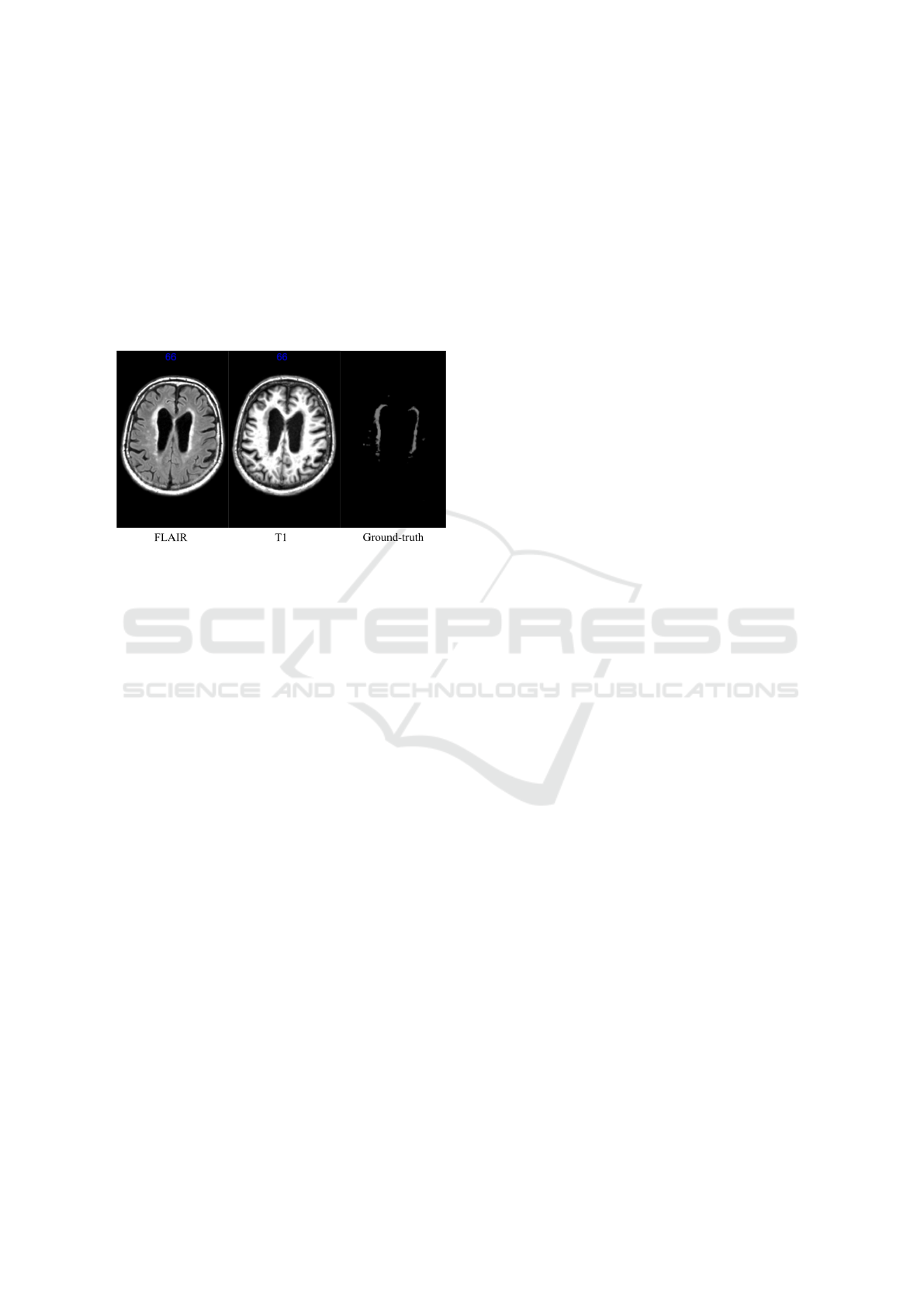
2.1 The Dataset
The images used for training and validation came
from a dataset provided by the MICCAI WMH Chal-
lenge (Kuijf et al., 2019), which consisted of images
of 60 subjects, acquired from three different 3T scan-
ners and places: Amsterdam (AMS GE3T), Utrecht,
and Singapore. Each scanner contributed with a set of
20 pairs of images per subject. Fig. 1, shows a sample
of the images.
Figure 1: Sample of one slice of the dataset used as input for
training. T1-weighted, FLAIR and a manually segmented
mask of the WMH (Ground-truth).
It is important to note that scanners and volun-
teers came from three different hospitals and MRI
scanners: two from the Netherlands and one from
Singapore. As described in (Kuijf et al., 2019), the
parameters’ settings of the acquisition images like
voxel size, slice number, and echo time were differ-
ent for each scanner. The images acquired per subject
were: 3D-T1-weighted images and 2D-multi-slice
FLAIR images. Further, the provided images were
pre-processed previously to correct the bias field in-
homogeneities, re-sampled, and coregistered between
them using SPM12 software. Additionally, the con-
test provided the ground-truth images obtained from
each FLAIR image, which were manually segmented.
The segmentation was done by two expert observers,
O1 and O2. The process was made following the
STandards for ReportIng Vascular changes on nEu-
roimaging (STRIVE) conventions (Wardlaw et al.,
2013) — the observer O1 segmented all images using
a contour drawing technique delineating the outline
of each WMH. The second observer O2 performed a
peer review over the manual delineations of O1, fol-
lowing a peer project methodology. A detailed de-
scription of the manual segmentation can be found in
(Kuijf et al., 2019). These images contained binary
masks of the WMH lesions, which correspond to the
ground-truth.
Additionally, the organizers kept in reserved 110
cases from five different scanners; these images were
not provided to the participants. 30 out of the 110
cases, were from each of the scanners mentioned be-
fore, and 20 from two additional scanners (from Am-
sterdam, but with different characteristics, such as
less magnetic field strength). All of these images
were also pre-processed using the same procedure de-
scribed before. The contest reserved these images for
testing purposes and metrics calculation.
2.2 Data Preparation and Further
Pre-processing
Before training the model, data from all sources were
merged into one dataset, consisting of 60 pairs of im-
ages: one T1-weighted image and FLAIR per subject.
All slices for each image were resized to 200x200
pixels across the y and z axis, using the numpy li-
brary in python. Further, we selected a field of view
from all images that contained the brain, cropping
the volume to discard the neck. We also performed
additional pre-processing procedures on all images;
such as, a Gaussian normalization to reduce noise,
highlight small brightness spots and smooth the im-
ages, and a morphological normalization to reduce
the black and low-intensity brain regions produced by
cerebral atrophy. This morphological normalization
was performed with the scipy python library.
2.3 Data Augmentation
To prevent the model from overfitting and to increase
the size of the training and testing datasets, we ap-
plied some data augmentation strategies with two ap-
proaches. The first includes standard operations, like
rotation, scaling, and shearing to all images. Each
transformation increased up to 60 additional images
to the original dataset, increasing from 60 to 240
images for each MRI channel. We also included
more complex data augmentation procedures; such as,
linear and nonlinear transformations over the origi-
nal data. For the linear transformations, we used a
pointwise product between the FLAIR and T1 im-
ages. And, we applied a diffeomorphic transforma-
tion for the nonlinear data augmentation, normaliz-
ing from the native space to the MNI 152 standard
space (Fonov et al., 2011; Fonov et al., 2009), using
the nipype library. After these procedures, we created
a separate dataset with the linear and nonlinear trans-
formations.
2.4 Network Architecture
The proposed model’s architecture was designed to
use two types of images as input per subject: T1-
HEALTHINF 2021 - 14th International Conference on Health Informatics
246
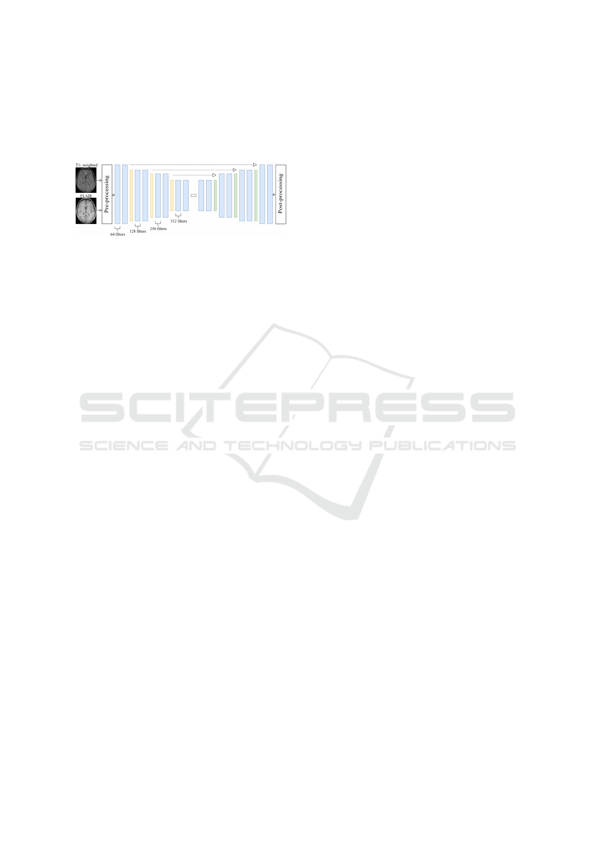
weighted and FLAIR images with the correspond-
ing pre-processed procedures explained before. Addi-
tionally, both images need to be coregistered between
them, including a field bias inhomogeneities correc-
tion.
Figure 2: U-Net Neural Network Architecture.
For this research, we designed three different seg-
mentation models based on a fully CNN architec-
ture, as proposed by (Long et al., 2014; Milletari
et al., 2016); and, in particular the U-net architec-
ture (Ronneberger et al., 2015b), which had proven
to be highly useful in biomedical image segmenta-
tion. In this work, the U-Net architecture performed
the best, a model with 21 layers, including 15 con-
volutional layers, three upsampling layers, and three
pooling layers. Fig. 2 shows a general representation
of this model’s architecture. For the first two layers
we used 5x5 convolutional filters, while for the rest a
set of 3x3 convolutional filters were used. After each
convolutional layer, a Rectified Linear Unit (RELU)
activation function was applied (Agarap, 2018). The
yellow boxes in Fig. 2 represent the max pooling or
downsamplig procedures, and the green boxes the up-
sampling operation, both with 2x2 filters. The num-
ber of filters in each layer goes from 64 in the two first
convolutional layers to 128, 256, and 512 filters in the
left side of the U-Net. We use Adam Stochastic Gra-
dient Descent for the learning process of the model
(Kingma and Ba, 2014). The learning rate was set to
0.0002. The training was performed with 30 batches,
and the parameter’s search was performed during 50
epochs. The other two models were designed with a
similar configuration, but with some modifications of
the hyper-parameters, as discussed in the next section.
Once the models were trained, cross-validated and
tested, the models were put into an inference stage,
where the architectures were also tested with new T1
and FLAIR images, which were not seen during the
previous phases, to let them recognize the WMH le-
sions, as well as to perform the segmentation in the
images.
2.5 Evaluation
The models were evaluated using six metrics as
defined by the MICCAI WMH segmentation chal-
lenge. Those metrics were: Dice Similarity Coeffi-
cient (DSC), Hausdorff Distance (HD), Average Vol-
ume Difference (AVD), Sensitivity for detecting indi-
vidual lesions, (Recall), and the F1-score. The Dice
similarity metric measures the overlap between the
manual segmentation and the model segmentation.
The Hausdorff Distance measures how far two sub-
sets of a metric space are from each other. As used in
this challenge, the Hausdorff Distance is modified as
to obtain the most robust version using the 95th per-
centile instead of the maximum 100th percentile dis-
tance. The Average Volume Difference metric mea-
sures the percentage difference in the volume of the
manual segmentation lesions compared to the model
segmentation. As for the Recall metric, this measures
the ability of a model to find all relevant cases within
the data. And, the F1 index is a way to combine the
recall with its precision, which is defined as the har-
monic mean of both, as defined in (Li et al., 2018b).
The model evaluation was performed in two parts.
First, a local testing was made using the three differ-
ent U-nets architectures, tuning the hyper-parameters
to push for the ground-truth masks and for the met-
rics obtained by the 2017’s challenge winner (Li et al.,
2018b). Then, once our best model was tuned for the
best performance, it was evaluated by the WMH chal-
lenge organizers, using their own additional test im-
ages, which placed our architecture ninth on the over-
all challenge up to November 2020.
3 RESULTS AND DISCUSSION
3.1 Local Results
Before configuring our three U-Net based models, we
evaluated the Re f erence models, to set the basis for
comparing our models. We evaluated the model pre-
sented by (Li et al., 2018b), which was taken as refer-
ence. Then, the challenge’s Re f erence model, which
we use it to obtain the metrics as described by the
challenge. Based on these baseline architectures, our
first proposed model was created based on the U-net
architecture as shown in Fig. 2; this first model was
called (U − net#1), and its architecture was config-
ured to take two channels as input: a FLAIR image
and an augmented image obtained by a dot product
of the T1 and the FLAIR. This architecture produced
low performance as compared to the reference mod-
els and did not require further analysis.
Automatic Brain White Matter Hypertinsities Segmentation using Deep Learning Techniques
247
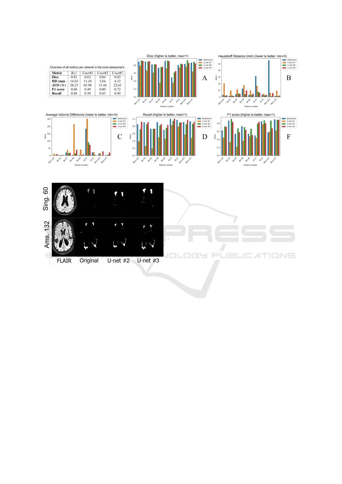
Figure 3: General results of the internal testing.
Figure 4: Figure shows a comparison of the same slice of
two images between the ground-truth (Original) and auto-
matic segmentation performed by U −net#2 and U −net#3.
Then a second model was configured, which we
called (U − net#2), and it was tune-designed to ac-
cept our pre-processed FLAIR and T1 images as in-
puts, which was defined in our pre-processing phase,
with promising results. Fig. 3 shows the segments
obtained by this models as compared to the original
or ground-truth.
A third model then was evaluated, a model called
(U − net#3), which was designed to use an Exponen-
tial Linear Unit ELU (Clevert et al., 2015), as ac-
tivation function in the convolutional steps, and the
he − normal as kernel initializer (He et al., 2015)
in the last step. This model performed better than
the reference, but not as good as the model called
U − net#2. Fig. 4 also shows the segments obtained
by this models as compared to the original or ground-
truth.
Therefore, our second model was uploaded to the
WMH challenge platform. Figures 3 and 5 show the
results of the testings performed locally and the re-
sults assessed by the WMH organizers.
For local testing purposes, eight images were se-
lected randomly and used to compare the resulting
segments from the four models. The eight images
were obtained from the three scanners proportionally,
making sure to have at least two subjects for the input
scanner. The metrics used in the local testing were
the same as they were defined by the challenge orga-
nizers; that is, the Dice, Hausdorff Distance, Average
Volume Difference, F1 score, and Recall. The results
could be seen in Fig. 3. This figure shows a gen-
eral summary of all metrics assessed locally in our
experiments. The Ams prefix are patients from the
Amsterdam scanner, Sin is from the Singapore scan-
ner, and Ut is from the Utrecht scanner. Additionally,
the table in Fig. 3, shows the average results for all
metrics from each model. Fig. 4 shows the segments
from two MRI images: Singapore (subject #60) and
Amsterdam (subject #132). The original label is the
manual segmentation done by experts and provided
by the challenge organizers. As it is shown in Fig. 4,
our U − net#2 and U − net#3 models obtained com-
parable segmentation results as to the experts’ defined
segments.
As it is seen in Fig. 3A, the Dice metric, in our
U − net#2 and #3 models, performed better than the
Re f erence model. Also, the performance gain was
in general better. These metrics were 4.84% and 3%,
respectively better than the Re f erence model.
On the other hand, the Hausdorff distance, as seen
in Fig. 3B, was significantly better. For example,
a subject from the Amsterdam group has a Hausdorff
Distance of 65.52 mm in the Re f erence segmentation.
While in model U − net#2, such difference reached
HEALTHINF 2021 - 14th International Conference on Health Informatics
248

0.98 mm, which represents an improvement of 67.10
times over the actual Re f erences. On average, the
Hausdorff Distance between the manual segmenta-
tion and the automatic segmentation, obtained in this
work, was 4.62 times better than the Re f erence.
The Average Volume Difference is observed in
Fig. 3C. In this metric, we obtained more varia-
tion. For example, in two patients from the Amster-
dam scanner, the U −net#2 performed better than the
rest of the models. The U − net#3 worked very well
on images from the Utrecht scanner. However, in gen-
eral, both the U − net#2 and #3 performed better seg-
menting than the Re f erence. While the average AV D
of the validation patients in the Re f erence model was
28.23 % in our model U − net#2 was 15.44 %and
22.63 % in the U − net#3. Although, Both methods
performed better compared to the Re f erence model.
The F1 score can be seen in Fig. 3F. The aver-
age value of the eight validation subjects’ images was
0.68, while our score was 0.80. In absolute terms, the
U −net#2 improved 17.3 % and the U −net#3, 6.16%
as compared to the Re f erence.
Finally, the recall metric can be seen in Fig. 3D.
This metric was the only one which did not im-
prove, as compared to the Re f erence models using
the U − net#2 model. In average the value obtained
with our model was 0.83, while the Re f erence model
was 0.88. However, the U −net#3 performed better in
the recall metric, we obtained 0.90, representing 1.3%
improvement as compared to the re f erence model.
3.2 WMH Validations
In this section, we present a summary of the evalu-
ations made by the WMH challenge organizers. The
model submitted to evaluation was the U −net#2. The
evaluation method is based on the rankings of each
metric, as described before, using a score from 0 to
1. The best performing team is ranked with 0 and
the worst with 1. All other teams were ranked in be-
tween relative to their performance within that met-
ric range. Then to compute the final score, the five
ranks were averaged in an overall final score, as de-
scribed in (WMH Segmentation Challenge, 2020). In
general, this work was placed ninth out of 43 partici-
pant teams, and as reported in November 2020, with
a score of 0.0596. Even though the metrics mea-
sured locally favored us, we could not improve the
Re f erence performance with the organizers’ assess-
ment, as observed in the results section of the web
site: (https://wmh.isi.uu.nl). A summary of this re-
sults can be seen in Fig. 5. Each figure includes a box
plot for every metric against the scanners tested by the
organizers. It is important to note, that the organizers
tested with images acquired from scanners with a dif-
ferent technology than the used for our training pro-
cess, as it is seen in the table, in Fig. 5. All the images
provided by the contest were obtained by different
brands of 3 Tesla scanners. However for validation
purposes, the contest also included images obtained
from 1.5 Tesla (AMS GE1.5T) and a hybrid Positron
Emission Tomography/MRI (AMS PETMR). The or-
ganizer’s results includes the average for each scan-
ner and the ranking of each metric against the other
teams, our worst results are observed precisely for the
AMS GE1.5T and AMS PETMR, images from scan-
ners with different technology not used for training.
The Dice metric performed best for Singapore
subjects. All validation results seem to have some
standard deviation and outliers, considering the im-
ages’ origin. In our case, the Singapore patients and
the AMS GE3T patients have a Dice score of 0.80 and
0,79, respectively, demonstrating good performance.
The Dice score, however, for the AMS PETMR was
slightly lower, with a 0.71 value, than the rest of the
scanners.
As for the Hausdorff distance metric, our model
performed particularly good; in this metric our model
was placed in fifth place with an overall rank of 0.017.
We also obtained a slightly better result in this met-
ric than the Re f erence, with an averaged distance of
6.30 mm, as compared to ours of 6.24 mm. The image
shows that the distance is almost always below the 20
mm mark, with some outliers reaching 40 mm.
In the average volume difference metric, the aver-
age value with all the testing patients was 28.26 %.
The performance was good in nearly all the scanners
except the AMS PEMTR scanner, in that case, the av-
erage volume difference was 60.79 %.
Considering the recall, the results obtained from
the Amsterdam images were above 0.80. However,
with the Utrecht images, we obtained a score of 0.71.
Also, it is noticeable that in this work, the perfor-
mance was better for the exclusive training scanners,
in which the other metrics did not perform well. Over-
all, for the local testing, the recall was the weakest
metric obtained in our model, with an overall rank-
ing of 0.137 compared to the other teams. However,
the score of 0.78 was not as far from the 0.87, which
is the current higher score obtained up to November
2020.
Finally, the F1 score had an average value of 0.74.
This metric was the one with a more standard devia-
tion. All the scanners had averaged performances be-
tween 0.7 and 0.8, except for the AMS PETMR scan-
ner with 0.65.
Automatic Brain White Matter Hypertinsities Segmentation using Deep Learning Techniques
249
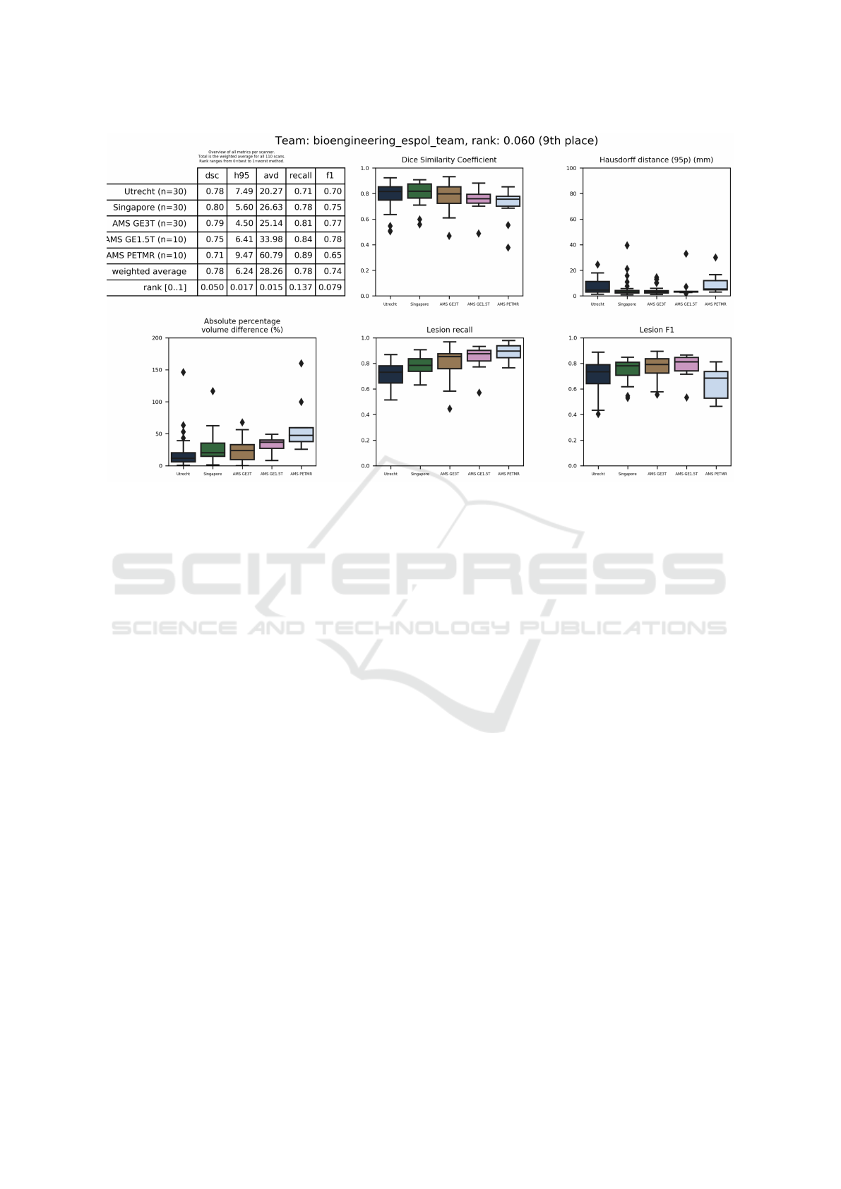
Figure 5: Overall results assessed by WMH challenge organizers.
3.3 Conclusions
We developed and evaluated a Convolutional Network
architecture for segmenting automatically WMH,
from FLAIR and T1 images. In our local evalua-
tions, we obtained and improvement in 4 out of 5 met-
rics, as defined by the WMH segmentation challenge.
That includes Dice, Hausdorff Distance, F1 score, and
Average Volume Difference. We were ranked ninth
place overall in the organizers’ assessment, obtaining
the best metric for the Hausdorff distance. As it can
be seen, our worst performance was with the images
coming from scanners not used during training, which
could be interpreted as over-fitting the data. How-
ever, considering a good performance obtained with
this proposed architecture, the hyper-parameter tun-
ing and the re-training of the algorithm, with images
from additional scanners technology could improve
the algorithm performance. Therefore, the work pre-
sented here could lead to other researchers to improve
the state of the art, for all society’s benefit.
ACKNOWLEDGEMENTS
We thank the MICCAI-2017 WMH Challenge orga-
nizer Dr. Hugo J. Kuijf to share us all the datasets
of images and making all the validation results. We
also thank Phd. Luis Mendoza for the supervision of
the project work and Kevin Cando as this work was
initialized by him as his final degree project.
REFERENCES
Abadi, M., Barham, P., Chen, J., Chen, Z., Davis, A.,
Dean, J., Devin, M., Ghemawat, S., Irving, G., Isard,
M., et al. (2016). Tensorflow: A system for large-
scale machine learning. In 12th {USENIX} Sympo-
sium on Operating Systems Design and Implementa-
tion ({OSDI} 16), pages 265–283.
Agarap, A. F. (2018). Deep learning using rectified linear
units (relu).
Ashburner, J. and Friston, K. J. (2005). Unified segmenta-
tion. Neuroimage, 26(3):839–851.
Bento, M., de Souza, R., Lotufo, R., Frayne, R., and Rittner,
L. (2017). Wmh segmentation challenge: A texture-
based classification approach. In International MIC-
CAI Brainlesion Workshop, pages 489–500. Springer.
Berseth, M. (2017). Wmh segmentation challenge, miccai
2017.
Breteler, M., van Swieten, J. C., Bots, M. L., Grobbee, D.
E., Claus, J. J., van den Hout, J. H., van Harskamp, F.,
Tanghe, H. L., de Jong, P. T., van Gijn, J., and Hof-
man, A. (1994). Cerebral white matter lesions, vascu-
lar risk factors, and cognitive function in a population-
based study. 44(7):1246–1246.
Chancay, O., Haro, T., Yapur, M., Alvarado, R., Pastor, M.,
and Loayza, F. (2015). Nuevo biomarcador en la en-
fermedad de parkinson mediante el an
´
alisis y cuan-
tificaci
´
on de lesiones cerebrales en secuencias flair
obtenidas por resonancia magn
´
etica (acl-tool). Revista
Tecnol
´
ogica-ESPOL, 28(5).
HEALTHINF 2021 - 14th International Conference on Health Informatics
250

Chollet, F. et al. (2015). Keras. https://github.com/ fchol-
let/keras, Sidst set 30/01/2020.
Clevert, D.-A., Unterthiner, T., and Hochreiter, S. (2015).
Fast and accurate deep network learning by exponen-
tial linear units (elus).
Cocosco, C. A., Zijdenbos, A. P., and Evans, A. C. (2003).
A fully automatic and robust brain mri tissue classifi-
cation method. Medical image analysis, 7(4):513-527
Daliri, R., M. (2012). Automated diagnosis of alzheimer
disease using the scale-invariant feature transforms
in magnetic resonance images. J Med Syst, 36:995–
1000.
Fonov, V., Evans, A., McKinstry, R., Almli, C., and
Collins, D. (2009). Unbiased nonlinear average age-
appropriate brain templates from birth to adulthood.
NeuroImage, 47:S102. Organization for Human Brain
Mapping 2009 Annual Meeting.
Fonov, V., Evans, A. C., Botteron, K., Almli, C. R., McK-
instry, R. C., and Collins, D. L. (2011). Unbiased
average age-appropriate atlases for pediatric studies.
NeuroImage, 54(1):313 – 327.
Ghafoorian, M., Karssemeijer, N., Heskes, T., van Uden,
W. I., Sanchez, I. C., Litjens, G., de Leeuw, E. F., van
Ginneken, B., Marchiori, E., and Platel, B. (2017a).
Location sensitive deep convolutional neural networks
for segmentation of white matter hyperintensities. Sci-
ence Reports, 7.
Ghafoorian, M., Mehrtash, A., Kapur, T., Karssemeijer,
N., Marchiori, E., Pesteie, M., Guttmann, R. C.,
de Leeuw, F., Tempany, C., van Ginneken, B., Fe-
dorov, A., Abolmaesumi, P., Platel, B., and Wells,
M. W. (2017b). Transfer learning for domain adapta-
tion in mri: application in brain lesion segmentation.
MICCAI 2017, Part III. LNCS, 10435:516–524.
Giorgio, A. and De Stefano, N. (2013). Clinical use of brain
volumetry. Journal of Magnetic Resonance Imaging,
37(1):1–14.
Gorgolewski, K. J., Esteban, O., Burns, C., Ziegler, E.,
Pinsard, B., Madison, C., Waskom, M., Ellis, D. G.,
Clark, D., Dayan, M., Manh
˜
aes-Savio, A., Notter,
M. P., Johnson, H., Dewey, B. E., Halchenko, Y. O.,
Hamalainen, C., Keshavan, A., Clark, D., Huntenburg,
J. M., Hanke, M., Nichols, B. N., Wassermann, D.,
Eshaghi, A., Markiewicz, C., Varoquaux, G., Acland,
B., Forbes, J., Rokem, A., Kong, X.-Z., Gramfort, A.,
Kleesiek, J., Schaefer, A., Sikka, S., Perez-Guevara,
M. F., Glatard, T., Iqbal, S., Liu, S., Welch, D., Sharp,
P., Warner, J., Kastman, E., Lampe, L., Perkins, L. N.,
Craddock, R. C., K
¨
uttner, R., Bielievtsov, D., Geisler,
D., Gerhard, S., Liem, F., Linkersd
¨
orfer, J., Margulies,
D. S., Andberg, S. K., Stadler, J., Steele, C. J., Brod-
erick, W., Cooper, G., Floren, A., Huang, L., Gonza-
lez, I., McNamee, D., Papadopoulos Orfanos, D., Pell-
man, J., Triplett, W., and Ghosh, S. (2016). Nipype: a
flexible, lightweight and extensible neuroimaging data
processing framework in Python. 0.12.0-rc1.
He, K., Zhang, X., Ren, S., and Sun, J. (2015). Delving deep
into rectifiers: Surpassing human-level performance
on imagenet classification.
Jack, R. C., O’Brien, P. C., Rettman, D. W. and, S. M. M.,
Xu, Y., Muthupillai, R., Manduca, A., Avula, R., and
Erickson, B. J. (2001). Flair histogram segmentation
for measurement of leukoaraiosis volume. J. Magn.
Reson. Imaging, 14(6):668–676.
Jin, D., Xu, Z., Harrison, A. P., and Mollura, D. J. (2018).
White matter hyperintensity segmentation from t1 and
flair images using fully convolutional neural networks
enhanced with residual connections. In 2018 IEEE
15th International Symposium on Biomedical Imaging
(ISBI 2018), pages 1060–1064. IEEE.
Kingma, D. and Ba, J. (2014). Adam: A method for
stochastic optimization. International Conference on
Learning Representations.
Kuijf, H. J., Biesbroek, J. M., De Bresser, J., Heinen,
R., Andermatt, S., Bento, M., Berseth, M., Belyaev,
M., Cardoso, M. J., Casamitjana, A., et al. (2019).
Standardized assessment of automatic segmentation
of white matter hyperintensities and results of the
wmh segmentation challenge. IEEE transactions on
medical imaging, 38(11):2556–2568.
Li, H., Jiang, G., Zhang, J., Wang, R., Wang, Z., Zheng,
W.-S., and Menze, B. (2018a). Fully convolutional
network ensembles for white matter hyperintensities
segmentation in mr images. NeuroImage, 183:650–
665.
Li, H., Jiang, G., Zhang, J., Wang, R., Wang, Z., Zheng,
W.-S., and Menze, B. (2018b). Fully convolutional
network ensembles for white matter hyperintensities
segmentation in mr images. NeuroImage, 183:650 –
665.
Li, H., Zhang, J., Muehlau, M., Kirschke, J., and Menze,
B. (2018c). Multi-scale convolutional-stack aggrega-
tion for robust white matter hyperintensities segmen-
tation. In International MICCAI Brainlesion Work-
shop, pages 199–207. Springer.
Long, J., Shelhamer, E., and Darrell, T. (2014). Fully con-
volutional networks for semantic segmentation.
Lowekamp, B., Chen, D., Ibanez, L., and Blezek, D. (2013).
The design of simpleitk. Frontiers in neuroinformat-
ics, 7:45.
McKinney, W. et al. (2010). Data structures for statisti-
cal computing in python. In Proceedings of the 9th
Python in Science Conference, volume 445, pages 51–
56. Austin, TX.
Microsoft (2020). Nc-series. https://docs.microsoft.com/
en-us/azure/virtual-machines/nc-series, Sidst set
02/03/2020.
Milletari, F., Navab, N., and Ahmadi, S.-A. (2016). V-
net: Fully convolutional neural networks for volumet-
ric medical image segmentation.
Morel, B., Xu, Y., Virzi, A., G’eraud, T., Adamsbaum, C.,
and Bloch, I. (2016). A challenging issue: detection
of white matter hyperintensities on neonatal brain mri.
Proceedings of the Annual International Conference
of the IEEE Engineering in Medicine and Biology So-
ciety (EMBC), page 93–96.
Oliphant, T. E. (2006). A guide to NumPy, volume 1. Trel-
gol Publishing USA.
Ronneberger, O., Fischer, P., and Brox, T. (2015a). U-
net: Convolutional networks for biomedical image
segmentation. International Conference on Medical
Automatic Brain White Matter Hypertinsities Segmentation using Deep Learning Techniques
251

image computing and computer-assisted intervention,
page 234–241.
Ronneberger, O., Fischer, P., and Brox, T. (2015b). U-
net: Convolutional networks for biomedical image
segmentation.
Van Rossum, G. and Drake Jr, F. L. (1995). Python refer-
ence manual. Centrum voor Wiskunde en Informatica
Amsterdam.
Virtanen, P., Gommers, R., Oliphant, T. E., Haberland, M.,
Reddy, T., Cournapeau, D., Burovski, E., Peterson, P.,
Weckesser, W., Bright, J., van der Walt, S. J., Brett,
M., Wilson, J., Jarrod Millman, K., Mayorov, N., Nel-
son, A. R. J., Jones, E., Kern, R., Larson, E., Carey,
C., Polat,
˙
I., Feng, Y., Moore, E. W., Vand erPlas, J.,
Laxalde, D., Perktold, J., Cimrman, R., Henriksen,
I., Quintero, E. A., Harris, C. R., Archibald, A. M.,
Ribeiro, A. H., Pedregosa, F., van Mulbregt, P., and
Contributors, S. . . (2020). SciPy 1.0: Fundamental
Algorithms for Scientific Computing in Python. Na-
ture Methods.
Vrooman, H. A., Cocosco, C. A., van der Lijn, F., Stokking,
R., Ikram, M. A., Vernooij, M. W., Breteler, M. M.,
and Niessen, W. J. (2007). Multi-spectral brain tissue
segmentation using automatically trained k-nearest-
neighbor classification. Neuroimage, 37(1):71–81.
Wardlaw, J., Smith, E., Biessels, G., Cordonnier, C.,
Fazekas, F., Frayne, R., Lindley, R., O’Brien, J.,
Barkhof, F., Benavente, O., Black, S., Brayne, C.,
Breteler, M., Chabriat, H., DeCarli, C., Leeuw, F.-E.,
Doubal, F., Duering, M., Fox, N., and v, S. (2013).
Neuroimaging standards for research into small vessel
disease and its contribution to ageing and neurodegen-
eration. The Lancet Neurology, 12:822–838.
Waskom, M., Botvinnik, O., O’Kane, D., Hobson, P.,
Lukauskas, S., Gemperline, D. C., Augspurger,
T., Halchenko, Y., Cole, J. B., Warmenhoven, J.,
de Ruiter, J., Pye, C., Hoyer, S., Vanderplas, J., Vil-
lalba, S., Kunter, G., Quintero, E., Bachant, P., Mar-
tin, M., Meyer, K., Miles, A., Ram, Y., Yarkoni, T.,
Williams, M. L., Evans, C., Fitzgerald, C., Brian,
Fonnesbeck, C., Lee, A., and Qalieh, A. (2017).
mwaskom/seaborn: v0.8.1 (september 2017).
WMH Segmentation Challenge (2020). Evalua-
tion. https://wmh.isi.uu.nl/evaluation/, Sidst set
30/11/2020.
Xu, Y., G eraud, T., and Bloch, I. (September 2017a).
From neonatal to adult brain mr image segmentation
in a few seconds using 3d-like fully convolutional net-
work and transfer learning. Proceedings of the 23rd
IEEE International Conference on Image Processing
(ICIP), page 4417–4421.
Xu, Y., G
´
eraud, T., Puybareau,
´
E., Bloch, I., and Chazalon,
J. (2017b). White matter hyperintensities segmenta-
tion in a few seconds using fully convolutional net-
work and transfer learning. In International MICCAI
Brainlesion Workshop, pages 501–514. Springer.
Zhang, Y., Brady, M., and Smith, S. (2001). Segmen-
tation of brain mr images through a hidden markov
random field model and the expectation-maximization
algorithm. IEEE transactions on medical imaging,
20(1):45–57.
Zijdenbos, A. P. and Dawant, B. M. (1994). Brain seg-
mentation and white matter lesion detection in mr
images. Critical reviews in biomedical engineering,
22(5-6):401–465.
HEALTHINF 2021 - 14th International Conference on Health Informatics
252
