Mixed-Integer Constrained Grey-Box Optimization based on
Dynamic Surrogate Models and Approximated Interval Analysis
Mohamad Omar Nachawati
a
and Alexander Brodsky
b
Department of Computer Science, George Mason University, Fairfax, Virginia, U.S.A.
Keywords:
Constrained Optimization, Grey-Box Optimization, Interval Analysis, Mixed-Integer Programming,
Non-convex Optimization, Nonlinear Programming, Simulation Optimization, Surrogate-based
Optimization.
Abstract:
In this paper an algorithmic framework, called GreyOpt, is proposed for the heuristic global optimization of
simulations over general constrained mixed-integer sets, where simulations are expressed as a grey-box, i.e.
computations using a mix of (1) closed-form analytical expressions, and (2) evaluations of numerical black-
box functions that may be non-differentiable and computationally expensive. GreyOpt leverages the partially
analytical structure of such problems to dynamically construct differentiable surrogate problems for multiple
regions of the search space. These surrogate problems are then used in conjunction with a derivative-based
method to locally improve sample points in each region. GreyOpt extends Moore interval arithmetic for ap-
proximating the intervals of grey-box objective and constraint functions by fitting quadric surfaces that attempt
to roughly underestimate and overestimate embedded black-box functions. This serves as the foundation of a
recursive partitioning technique that GreyOpt uses to refine the best points found in each region. An experi-
mental study of GreyOpt’s performance is conducted on a set of grey-box optimization problems derived from
MINLPLib, where the ratio of black-box function evaluations to analytical expressions is small. The results of
the study show that GreyOpt significantly outperforms three derivative-free optimization algorithms on these
problems.
1 INTRODUCTION
This paper considers the problem of mixed-integer
constrained grey-box (MICGB) optimization,
namely, of a real objective f (x,y) subject to a
box-constrained, vector-valued constraint function
g(x,y), where vectors x and y represent real and
integer decision variables, respectively, as formally
defined in Section 2. This is under the assump-
tion that both f (x,y) and g(x,y) are provided as a
grey-box simulation, i.e. a computation using a mix
of (1) closed-form analytical expressions, and (2)
evaluations of numerical black-box functions that can
be non-differentiable and computationally expensive.
This class of problems can be viewed as a continuum
between white-box optimization, where f and g are
completely defined in closed analytical form, and
black-box optimization, where f and g are provided
as black-box functions.
a
https://orcid.org/0000-0001-6153-8152
b
https://orcid.org/0000-0002-0312-2105
MICGB optimization has a wide-range of real-
world applications across diverse commercial and in-
dustrial domains, such as logistics, manufacturing and
supply chain management. This class of optimiza-
tion problems also arise from the analysis of multi-
disciplinary performance models that combine com-
putationally expensive and/or data-driven simulations
of continuous physical processes with metrics and
constraints involving discrete and finite domain de-
cision variables stemming from business processes
ranging from product design to production planning
and scheduling (Brodsky et al., 2019). Accurate and
efficient analysis of these models is crucial for im-
plementing effective decision guidance (DG) systems
that support model-driven decision-making in these
domains. DG systems are a special class of decision
support systems (DSS) that process large amounts
of data and analyze mathematical models to provide
an iterative process of ranking, prioritizing, and sug-
gesting actionable recommendations to and collecting
feedback from decision-makers, with the goal of ar-
riving at the best course of action (Brodsky and Wang,
Nachawati, M. and Brodsky, A.
Mixed-Integer Constrained Grey-Box Optimization based on Dynamic Surrogate Models and Approximated Interval Analysis.
DOI: 10.5220/0010350100990112
In Proceedings of the 10th International Conference on Operations Research and Enterprise Systems (ICORES 2021), pages 99-112
ISBN: 978-989-758-485-5
Copyright
c
 2021 by SCITEPRESS – Science and Technology Publications, Lda. All rights reserved
99

2008; Nachawati et al., 2017).
Despite a growing body of literature on grey-
box optimization, today only black-box optimiza-
tion algorithms are generally available for optimiz-
ing MICGB problems. Depending on the complexity
of the problem, meta-heuristic black-box algorithms
can provide adequate quality solutions with a reason-
able level of computational effort Talbi (2013). For
problems involving computationally expensive sim-
ulations, surrogate-based black-box algorithms, such
as EGO (Jones et al., 1998), can find high quality so-
lutions with significantly fewer costly objective and
constraint function evaluations than non-surrogate
black-box algorithms. However, these methods alone
do not scale well for high-dimensional problems
(Gilboa et al., 2013).
Although significant progress has been made on
the development of black-box optimization algo-
rithms, as their name implies they make little to no use
of the partially-analytical structure of MICGB prob-
lems. In some cases it may be possible to reformu-
late grey- and black-box problems, ahead of time, into
highly accurate analytical surrogate problems. This
approach can take considerably more effort and can
result in highly specialized surrogate models that are
difficult to reuse and dynamically update (Mazum-
dar et al., 2019). However, for tightly-constrained
and non-convex MICGB problems, the reformulated
surrogate can then be optimized using efficient and
globally convergent global optimization algorithms
that otherwise would not be applicable to the original
MICGB problem.
To ensure global convergence without degenerat-
ing into a brute-force search, efficient global opti-
mization algorithms rely on the ability to efficiently
fathom large areas of the search space with the aim
of quickly finding areas that are likely to contain
global optima and avoiding areas that do not. Sev-
eral fathoming techniques have been proposed in
the literature, including those based on: (1) inter-
val arithmetic (Moore, 1966), (2) McCormick re-
laxations (McCormick, 1976), (3) α-convexification
(Androulakis et al., 1995), and (4) Lipschitz continu-
ity (Pint
´
er, 1997). However, because of the significant
limitations of the structure and behavior of problems
that can be fathomed, none of the techniques above
are generally applicable to MICGB optimization.
In recent years, researchers have attempted to
enhance surrogate-based methods by exploiting the
partially analytical structure of grey-box optimiza-
tion problems. ARGONAUT, proposed by Bouk-
ouvala and Floudas (2017), supports the classifica-
tion of individual objective and constraint functions
as either white- or black-box. The black-box func-
tions from the original problem are then replaced
with approximations to generate a surrogate problem,
which is repeatedly calibrated and then optimized us-
ing ANTIGONE, a global optimization solver orig-
inally developed by Misener and Floudas (2014).
DEFT-FUNNEL, proposed by Sampaio (2019), fol-
lows a similar approach to ARGONAUT for classi-
fying white- and black-box objective and constraint
functions, but uses a sequential quadratic program-
ming (SQP) method paired with a multi-level single
linkage (MLSL) method instead of performing global
optimization on the surrogate.
However, there are some significant limitations to
those approaches. The authors of ARGONAUT re-
port a significant computational overhead for model
calibration. This problem is perhaps exacerbated
by ARGONAUT’s coarse-grain classification of ob-
jective and constraint functions as either white- or
black-box. Specifically, ARGONAUT treats expres-
sions that are largely analytical, but involve a nested
black-box function evaluation as completely black-
box. Also, the use of ANTIGONE—a global opti-
mization solver—on every iteration against the sur-
rogate problem is not cheap and may be of little
use if the surrogate is not accurate. Finally, DEFT-
FUNNEL does not support mixed-integer grey-box
optimization, and, like ARGONAUT, it is also lim-
ited in its coarse-grain classification of objective and
constraint functions.
Addressing these limitations is precisely the fo-
cus of this paper. Specifically, we make two main
contributions. First, we propose GREYOPT, an algo-
rithmic framework for the heuristic global optimiza-
tion of MICGB problems. GREYOPT supports a more
precise expression of grey-box problems than ARG-
ONAUT and DEFT-FUNNEL, where the analytical
structure, if any, of each objective and constraint func-
tions is preserved. GREYOPT leverages the partially
analytical structure of such problems to dynamically
construct differentiable surrogate problems for multi-
ple regions of the search space. These surrogate prob-
lems are then used in conjunction with a derivative-
based method to locally improve sample points in
each region. GREYOPT extends Moore interval arith-
metic (Moore, 1966) for approximating the intervals
of grey-box objective and constraint functions. This
serves as the foundation of a recursive partitioning
technique that GREYOPT uses to refine the best points
found in each region.
Second, we conduct an experimental study of
GREYOPT’s performance on a set of 25 MICGB opti-
mization problems, where the ratio of black-box func-
tion evaluations to analytical expressions is small.
ICORES 2021 - 10th International Conference on Operations Research and Enterprise Systems
100

The test problems are derived from MINLPLib
1
by
replacing some nonlinear terms of the object and
constraint functions with calls to otherwise equiva-
lent black-box functions. We adopt an evaluation
methodology based on performance profiles (Dolan
and Mor
´
e, 2002) and data profiles (Mor
´
e and Wild,
2009). The results of the study show that GREYOPT
significantly outperforms three derivative-free opti-
mization algorithms on these problems.
The rest of this paper is organized as follows. In
Section 2 we formally describe the MICGB class of
optimization problems that GREYOPT is designed to
handle. In Section 3 we describe the GREYOPT algo-
rithmic framework for the heuristic global optimiza-
tion of MICGB problems. In Section 4 we present an
experimental study of GREYOPT’s performance. Fi-
nally, in Section 5 we conclude the paper with some
brief remarks on directions for future work.
2 PROBLEM FORMULATION
Without loss of generality, this paper considers
MICGB optimization problems of the following form:
minimize
x∈R
n
, y∈R
m
f (x, y) (1a)
subject to g
L
≤ g(x,y) ≤ g
U
(1b)
x
L
≤ x ≤ x
U
(1c)
y
L
≤ y ≤ y
U
(1d)
y ∈ Z
m
(1e)
where f : R
n
× R
m
→ R is the objective function to
be minimized, and where g : R
n
× R
m
→ R
q
is the
vector-valued function of constraints, bounded below
by g
L
∈ R
q
and above by g
U
∈ R
q
, and where x ∈ R
n
are the real decision variables bounded below by x
L
∈
R
n
and above by x
U
∈ R
n
, and where y ∈ R
m
are the
integer decision variables bounded below by y
L
∈ R
m
and above by y
U
∈ R
m
, and lastly where n,m, q ∈ N
0
.
Stochastic optimization problems can be handled
using the formulation above through the use of ex-
pected values and chance constraints (Charnes and
Cooper, 1959). A stochastic objective
˜
f (x, y,ξ),
where ξ is the vector of uncertainty, can be
transformed into the objective function f (x,y) ,
E(
˜
f (x, y,ξ)), i.e. its expected value. Stochastic con-
straints ˜g
L
≤ ˜g(x,y, ξ) ≤ ˜g
U
can be transformed into
the constraints g
L
≤ g(x, y) ≤ g
U
, where g(x, y) ,
P( ˜g
L
≤ ˜g(x,y,ξ) ≤ ˜g
U
), and where g
L
and g
U
are the
lower and upper bounds of the vector of probabilities
that the stochastic constraints hold.
1
URL: http://www.minlplib.org/
It is assumed that f (x,y) and g(x,y) are provided
as a factorized grey-box simulation over input vec-
tors x and y, formally expressed as a Wengert list
(Wengert, 1964) of K ∈ N assignments:
(e
i
, E
i
(a
i
))
K
i=1
(2)
where the computed values of f (x,y) and g(x,y)
correspond to values e
F
and e
G
, respectively, given
F,G ∈ [1,K], and where e
i
is a tensor of real-valued
elements, and where input a
i
is a sequence of zero
or more values, in any order, from the sequence
(e
1
,..., e
i−1
), and lastly where E
i
is one of the follow-
ing:
• a constant tensor of real-valued elements
• a tensor of real-valued elements composed of any
of the components of variables x and y or any of
the elements of tensors e
1
,..., e
i−1
• a closed-form analytical expression in terms of the
elements of input a
i
• an evaluation of a black-box function R
N
→ R
M
on input a
i
3 GREY-BOX OPTIMIZATION
This section describes the GREYOPT algorithmic
framework for the heuristic global optimization of
MICGB problems. The main idea behind GREYOPT
is two-fold. First, the partially analytical structure
of MICGB optimization problems is leveraged to dy-
namically construct differentiable surrogate problems
for different regions of the search space. These sur-
rogate problems are then used in conjunction with a
derivative-based method to locally improve sample
points in each region. Second, a recursive partitioning
technique with a fathoming heuristic based on an ap-
proximated interval analysis is used to refine the best
points in each region.
Assuming the compact interval notation of [x] ,
[x,x], where x and x are the lower and upper bounds
of interval [x], respectively, given a function f : R
n
→
R
m
, its interval extension (Moore, 1966) is a func-
tion [ f ] : [R]
n
→ [R]
m
such that for any input inter-
val [x] ∈ [R
n
] the resulting interval [ f ]([x]) bounds all
the points in the set { f (y) : ∀y ∈ [x]}. Moore inter-
val arithmetic provides interval extensions of many
standard arithmetic operations and functions that are
generally admitted in closed-form expressions. For
example, the addition of intervals [x] and [y] is de-
fined as [x] + [y] , [x
L
+ y
L
,x
L
+ y
L
]. For a general
function f : R
n
→ R
m
that can be defined in such
closed analytical form, its interval extension can be
Mixed-Integer Constrained Grey-Box Optimization based on Dynamic Surrogate Models and Approximated Interval Analysis
101

obtained by the recursive substitution of each oper-
ation and function with their respective interval ex-
tension. This is known as the natural interval exten-
sion (Moore, 1966). GREYOPT extends Moore inter-
val arithmetic for approximating the natural interval
extension of grey-box objective and constraint func-
tions by fitting quadric surfaces (see Equation 6 and
Figure 1) that roughly underestimate and overestimate
each embedded black-box function call.
The high-level pseudocode for GREYOPT is given
in Algorithm 1. For input, GREYOPT expects a tuple
p that fully describes the MICGB optimization prob-
lem:
p , he,F, G,x
0
,y
0
,x
L
,x
U
,y
L
,y
U
,g
L
,g
U
i (3)
where e is a Wengret list representing the factorized
grey-box simulation (see Equation 2), and where F
and G are indexes of e that correspond to the objective
function f (x,y) value and constraint function g(x,y)
value, respectively, and where x
0
and y
0
are the ini-
tial values for the decision variables, and where x
L
,
x
U
, y
L
, and y
U
are the upper and lower bounds of the
decision variables, and finally where g
L
and g
U
are
the upper and lower bounds of the constraint function
g(x,y).
The parameters of GREYOPT are denoted in this
section by MONOSPACED text. GREYOPT expects to be
provided a configuration of parameter values that de-
fine its run-time behavior. As an algorithmic frame-
work, each parameterization can be considered as a
particular algorithm of GREYOPT to run. Upon termi-
nation, GREYOPT returns the best point (x
∗
,y
∗
) found
during the search. As a heuristic algorithm, GREY-
OPT makes no guarantee that the point it returns is
either optimal or feasible, even if such a solution is
known to exist. The rest of this section describes the
essential steps of the GREYOPT in more detail.
LINE 1 of Algorithm 1—Initialization. For prob-
lem p, GREYOPT begins by calling the Initialize
routine, which returns (1) an initial champion point
(x
∗
,y
∗
) using the initial values (x
0
,y
0
) for the deci-
sion variables of problem p, and (2) a priority queue R
of regions. In the implementation of GREYOPT, if an
initial value is not provided for a real-valued decision
variable x
i
, the midpoint of its bounds
x
L
i
+x
U
i
2
is used.
For an integer-valued decision variable y
i
, the closest
integer to the midpoint within the bounds of the deci-
sion variable is used, i.e. b
y
L
i
+y
U
i
2
c or d
y
L
i
+y
U
i
2
e.
During the evaluation of the objective and con-
straint functions for initial values (x
0
,y
0
), GREY-
OPT records the execution time for each black-
box function call to determine whether a surrogate
function should be used. If the execution time,
in seconds, of a black-box function does not ex-
ceed BLACKBOX TIME THRESHOLD, then GREYOPT
Algorithm 1: GREYOPT.
Input: p
Output: x
∗
∈ R
n
,y
∗
∈ R
m
Method:
1 (x
∗
,y
∗
,R) ← Initialize(p)
2 i ← 0
3 do
4 r ← SelectRegion(R,i)
5 (x
∗
r
,y
∗
r
) ← Champion({r})
6 if x
L
(r) = x
U
(r) ∧ y
L
(r) = y
U
(r) then
7 goto LINE 25 of Algorithm 1
8 S
0
← Sample(r)
9 r ← Calibrate(r, S
0
)
10 S
1
← {}
11 foreach (x
0
,y
0
) ∈ S
0
do
12 ( ˜x, ˜y) ← Improve(r, x
0
,y
0
)
13 if SurrogateCompare(r, ˜x, ˜y, x
∗
r
,y
∗
r
)
then
14 if ˜y /∈ Z
m
where m , | ˜y| then
15 ( ˜x, ˜y) ← Repair(r, ˜x, ˜y)
16 if p is separable then
17 ( ˜x, ˜y) ← FixedImprove(p, ˜x, ˜y)
18 if Compare(p, ˜x, ˜y,x
∗
r
,y
∗
r
) then
19 S
1
← S
1
∪ ( ˜x, ˜y)
20 r ← UpdateChampion(r, ˜x, ˜y)
21 end
22 if |S
1
| > 0 then
23 R ← R ∪ Cluster(r,S
1
)
24 else
25 R ← R ∪ Refine(r,R)
26 while |R| > MAX REGION QUEUE SIZE do
27 R ← R \ {WorstRegion(R)}
28 end
29 i ← i + 1
30 (x
∗
,y
∗
) ← Champion(R)
31 while ¬Converged(R,i)
32 return (x
∗
, y
∗
)
will not generate surrogates for that function and its
derivatives will be approximated by finite differences.
In the implementation of GREYOPT, this feature can
be disabled by the user on a per-function basis. For
the rest of this section, we use the term black-box
function to refer exclusively to those whose deriva-
tives will not be approximated by finite differences,
unless otherwise noted. After initialization, GREY-
OPT iterates through lines 4-30 of Algorithm 1 until at
least one of the convergence criteria has been fulfilled
(see the description for LINE 31 of Algorithm 1).
The region queue R is initialized with the global
region object r
g
corresponding to the entire search
space of problem p. Region objects are used as an
intensification mechanism by GREYOPT to restrict
ICORES 2021 - 10th International Conference on Operations Research and Enterprise Systems
102

sampling and surrogate calibration to a specific area
of a problem’s search space. Formally, a region ob-
ject r is defined by a tuple:
r , h ˜p,i, x
∗
,y
∗
,x
L
,x
U
,y
L
,y
U
i (4)
where ˜p is the region’s surrogate problem, and where
i is the region’s iteration count, and where (x
∗
,y
∗
) is
the region’s champion point (i.e. the best point found
in that region), and where x
L
, x
U
, y
L
, and y
U
are the
upper and lower bounds of the decision variables for
the region. The surrogate problem ˜p is obtained by
replacing all the black-box functions of the original
problem p with surrogate functions that are calibrated
using all the sample points that fall within the bounds
of the region (see the description for LINE 9 of Algo-
rithm 1).
LINE 4 of Algorithm 1—Region Selection. At the
start of each iteration, GREYOPT selects and removes
a region r from the front of region queue R, and in-
crements the iteration count i of region r. To balance
exploration versus exploitation, regions within R are
first ordered by the iteration count i, and then by the
fitness of its champion point (x
∗
,y
∗
). GREYOPT uses
the comparison function in Algorithm 2 to compare
the fitnesses of two points (x
0
,y
0
) and (x
1
,y
1
), where
the Evaluate function computes the objective value f ,
the constraint values vector g, and the constraint vio-
lation vector v for a point (x, y) in the search space of
problem p.
Algorithm 2: Comparison.
1 function Compare(p,x
0
,y
0
,x
1
,y
1
)
2 m ← |y
0
|
3 ( f
0
,g
0
,v
0
) ← Evaluate(p, x
0
,y
0
)
4 ( f
1
,g
1
,v
1
) ← Evaluate(p, x
1
,y
1
)
5 if kv
0
k
2
= 0 then
6 if kv
1
k
2
> 0 then
7 return true
8 if y
0
∈ Z
m
then
9 if y
1
/∈ Z
m
then
10 return true
11 else if y
1
∈ Z
m
then
12 return false
13 return f
0
< f
1
14 if kv
1
k
2
= 0 then
15 return false
16 return kv
0
k
2
< kv
1
k
2
17 end
LINE 8 of Algorithm 1—Sampling. For each iter-
ation, GREYOPT randomly samples a set S
0
of points
within the bounds of the selected region r. If the prob-
lem has no black-box functions then only one point
is randomly sampled per iteration, otherwise the to-
tal number of points to sample is determined by the
MAXIMUM SAMPLES PER ITERATION parameter.
Samples are drawn by alternating between two
different sampling distributions: (1) a uniform
distribution U(a, b), where a , (x
L
,y
L
) and b ,
(x
U
,y
U
), and (2) a modified-PERT distribution
MPERT (a,b,c,γ), where a , (x
L
,y
L
), b , (x
∗
,y
∗
),
c , (x
U
,y
U
), and γ , (x
U
− x
L
,y
U
− y
L
). For integer-
valued decision variables, the closest integer to the
sampled value within the bounds of the decision vari-
able is selected. The rationale behind the use of the
two distributions is to balance between sample point
diversity that is provided by the uniform distribution,
and sample point intensification around the current
champion point (x
∗
,y
∗
) of region r that is provided
by the modified-PERT distribution.
Definition 3.1 (White-box Constraint). Let p be a
MICGB problem with vector-valued constraint func-
tion g(x,y). We say that a component g
i
∈ g(x,y) is
a white-box constraint if and only if its computation
does not entail any call to a black-box function.
Definition 3.2 (Restorable Problem). Let p be a
MICGB problem with vector-valued constraint func-
tion g(x,y). We say that p is a restorable problem if
and only if there exists a component g
i
∈ g(x,y) that
is a white-box constraint.
For highly constrained problems, it is unlikely that
any sample point (x
0
,y
0
) will be feasible. If the prob-
lem is restorable, GREYOPT tries to find the clos-
est point (x,y) that satisfies all white-box constraints
g
i
∈ g(x,y) by solving the following restoration prob-
lem:
minimize
x∈R
n
, y∈R
m
kx
0
− xk
2
+ ky
0
− yk
2
(5a)
subject to w
L
≤ w(x,y) ≤ w
U
(5b)
x
L
≤ x ≤ x
U
(5c)
y
L
≤ y ≤ y
U
(5d)
y ∈ Z
m
(5e)
where (x
0
,y
0
) is the sample point to restore, and
where (x,y) are the decision variables representing
the restored point, and where w : R
n
× R
m
→ R
q
is
the vector-valued function of white-box constraints
that is obtained from g(x,y) of the original problem
by removing all components g
i
∈ g(x,y) that are not
a white-box constraint, and where w(x, y) is bounded
below by w
L
∈ R
q
and above by w
U
∈ R
q
. If success-
ful, the original sample point (x
0
,y
0
) is replaced by
the restored point (x,y).
LINE 9 of Algorithm 1—Calibration. The
Calibrate routine constructs and calibrates a surro-
gate problem ˜p for region r by replacing each call
Mixed-Integer Constrained Grey-Box Optimization based on Dynamic Surrogate Models and Approximated Interval Analysis
103

(a) Interval [-10, 10]. (b) Interval [-5, 5].
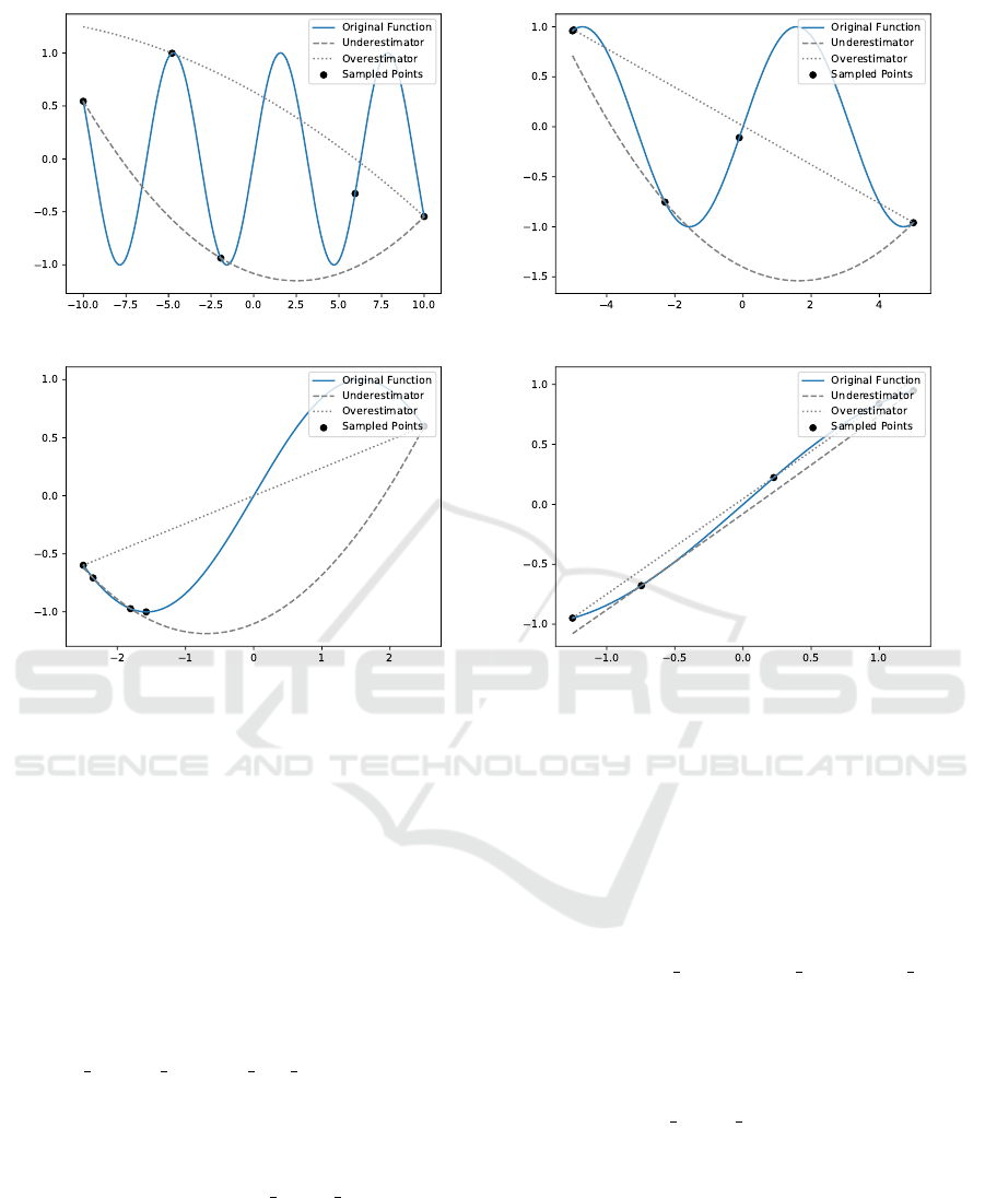
(c) Interval [-2.5, 2.5]. (d) Interval [-1.25, 1.25].
Figure 1: Plots of sin(x) versus quadric surrogates used as a rough underestimator and overestimator that is fitted based on
three randomly sampled points, plus the limit points, over increasingly smaller intervals.
to a black-box function B in the original problem
with a call to a corresponding surrogate function.
For each black-box function B, the upper and lower
bounds of region r are projected onto the domain of
the B using the approximated interval arithmetic de-
scribed at the beginning of this section. The pro-
jected upper and lower bounds of the domain of B
in region r are used to select a subset S
B
of previ-
ously evaluated input and output values for B from
a cache that is maintained for each black-box func-
tion. The size of this cache is controlled by the
MAXIMUM CACHED SAMPLES PER FUNCTION parame-
ter. If a surrogate function has already been con-
structed and calibrated for B in region r, the coef-
ficient of determination, i.e. R
2
score, is computed
using set S
B
. If the R
2
score of the surrogate func-
tion falls below CALIBRATION
SCORE THRESHOLD, it
is replaced by a new surrogate function that is cali-
brated using set S
B
. Otherwise, the previously cali-
brated surrogate function is reused for the remainder
of the current iteration.
A simple model selection method on an ordered
set of candidate surrogate models is used to au-
tomatically choose a surrogate function for black-
box function B . In the implementation of GREY-
OPT the following two regression models, provided
by scikit-learn (Pedregosa et al., 2011), are con-
sidered for model selection: (1) a polynomial re-
gression model using a combination of polynomial
features, where the maximum degree is controlled
by the MAXIMUM POLYNOMIAL SURROGATE DEGREE
parameter, and (2) a Gaussian process regression
(GPR) model with a radial basis function (RBF)
kernel. The polynomial model is first calibrated
and scored using set S
B
of input and output val-
ues. If its R
2
score is greater than or equal
to CALIBRATION SCORE THRESHOLD, then the cali-
brated polynomial model is chosen. Otherwise the
GPR model is calibrated and scored using S
B
, and the
model with the best R
2
is chosen.
To calibrate the quadric surface used to approxi-
mately underestimate a black-box function B : R
n
→
R
m
, the following constrained regression problem is
ICORES 2021 - 10th International Conference on Operations Research and Enterprise Systems
104

Algorithm 3: Refinement.
1 function Refine(r,R)
2 (x
∗
,y
∗
) ← Champion(R)
3 R
∗
← {}
4 c ← 0
5 R
c
← {ExpandChampion(r,c)}
6 while |R
c
| > 0 do
7 r
c
← RefinementRegion(R
c
)
8 x
∆
← kx
U
(r
c
) − x
L
(r
c
)k
∞
9 y
∆
← ky
U
(r
c
) − y
L
(r
c
)k
∞
10 σ ← min{ε,
MINIMUM PARTITION SIZE
10
c
}
11 if x
∆
≤ σ ∧ y
∆
≤ σ then
12 R
∗
← R
∗
∪ {r
c
}
13 if |R
∗
| ≥ MAX REFINES then
14 break
15 else
16 x
m
←
x
L
(r
c
)+x
U
(r
c
)
2
17 y
m
←
y
L
(r
c
)+y
U
(r
c
)
2
18 ( f
c
,g
c
) ← Evaluate(p, x
m
,y
m
)
19 if ¬Validate(r
c
, f
c
,g
c
) then
20 r
c
← CalibrateQuadric(r
c
)
21 (r
0
,r
1
) ← Partition(r
c
)
22 if RegionCompare(r
0
,x
∗
,y
∗
) then
23 R
c
← R
c
∪ {r
0
}
24 if RegionCompare(r
1
,x
∗
,y
∗
) then
25 R
c
← R
c
∪ {r
1
}
26 while |R
c
| > CACHED REGIONS do
27 R
c
← R
c
\ {WorstRegion(R
c
)}
28 end
29 c ← c + 1
30 if c >= ITERATION LIMIT then
31 break
32 end
33 if r is the global region then
34 R
∗
← R
∗
∪ {r}
35 else if |R
∗
| = 0 then
36 if RegionCompare(r,x
∗
,y
∗
) then
37 R
∗
← R
∗
∪ {r}
38 return R
∗
39 end
solved:
minimize
A,B,C
kY − (AX
◦2
+ BX +CJ)k
2
(6a)
subject to Y − (AX
◦2
+ BX +CJ) ≥ ε (6b)
∀i ∀ j, A
i j
≥ ε (6c)
where A ∈ R
m×n
, B ∈ R
m×n
, C ∈ R
m×1
are the coef-
ficients of the quadric surface, where J ∈ {1}
1×s
is a
unit matrix, where X ∈ R
n×s
and Y ∈ R
m×s
are the
input and output values of S
b
in matrix form, where s
is the number of samples in S
B
, and where
◦
is used
to denote element-wise exponentiation. A small pos-
itive number constant, ε, is used (1) to ensure that
the quadric surface is never greater than any of the
output values contained in S
B
(Equation 6b), and (2)
to ensure the convexity of the quadric surface (Equa-
tion 6c).
The quadric surface for approximately overesti-
mating a black-box function B is calibrated in a sim-
ilar fashion, except the inequalities in Equation 6 are
reversed. Figure 1 shows some plots of sin(x) ver-
sus quadric surrogates used as a rough underestima-
tor and overestimator that is fitted based on three ran-
domly sampled points, plus the limit points, over in-
creasingly smaller intervals.
LINES 10-21 of Algorithm 1—Improvement.
With the surrogate problem ˜p of region r constructed,
GREYOPT tries to locally improve each sample point
(x
0
,y
0
) ∈ S
0
. The Improve routine runs a derivative-
based convex nonlinear optimization solver on ˜p with
a starting point of (x
0
,y
0
). In the implementation of
GREYOPT, the open-source solver IPOPT (W
¨
achter
and Biegler, 2006) is used with a max cpu time of
IMPROVE TIME LIMIT FACTOR × (n + m + q) (7)
where n, m, and q are the number of variables (real-
and integer-valued) and constraints of the problem p
(see the MICGB formulation in Equation 1).
On Line 13 of Algorithm 1, the call to the
SurrogateCompare function compares the surrogate
fitnesses of points ( ˜x, ˜y) and (x
∗
r
,y
∗
r
) using the surro-
gate problem of region r, and returns true if ( ˜x, ˜y)
is better than (x
∗
r
,y
∗
r
), and false otherwise. The
SurrogateCompare function is similar to the compar-
ison function in Algorithm 2), except that it uses the
surrogate problem of region r to evaluate the objec-
tive value f and constraint violations vector v, and it
relaxes the requirement for integer feasibility.
On Lines 14-15 of Algorithm 1, if the point ( ˜x, ˜y)
is not integer feasible, the Repair routine runs a
derivative-based, mixed-integer convex nonlinear op-
timization solver on ˜p with a starting point of ( ˜x, ˜y) to
try to achieve integer feasibility. In the implementa-
tion of GREYOPT, the open-source solver BONMIN
(Bonami et al., 2008) is used with a time limit of
REPAIR TIME LIMIT FACTOR × (n + m + q) (8)
where n, m, and q are the number of variables (real-
and integer-valued) and constraints of the problem p
(see the MICGB formulation in Equation 1).
Definition 3.3 (White-box Decision Variable). Let p
be a MICGB problem with decision variables (x,y).
We say that a real-valued decision variable x
i
∈ x or
an integer-valued decision variable y
i
∈ y is a white-
box decision variable if and only if that variable does
Mixed-Integer Constrained Grey-Box Optimization based on Dynamic Surrogate Models and Approximated Interval Analysis
105

not contribute to the input of any black-box function
called for the computation of the objective and con-
straint functions of p.
Definition 3.4 (Separable Problem). Let p be a
MICGB problem with decision variables (x,y). We
say that p is a separable problem if and only if there
exists a real-valued decision variable x
i
∈ x or an
integer-valued decision variable y
i
∈ y that is white-
box.
On Lines 16-17 of Algorithm 1, if problem p is
separable, the FixedImprove routine runs a derivative-
based, mixed-integer convex nonlinear optimization
solver on the original problem p with a starting point
of (˜x, ˜y). Unlike with the Improve routine, which uses
the original decision variable bounds of the problem
p, the FixedImprove routine fixes the bounds of all
decision variables that are not white-box to the values
of the champion point (x
∗
r
,y
∗
r
). To prevent costly re-
evaluations of black-box functions, GREYOPT caches
and recalls the last evaluated point for each black-box
function call while running FixedImprove.
On Line 18 of Algorithm 1, the call to the
Compare function compares the fitnesses of points
( ˜x, ˜y) and (x
∗
r
,y
∗
r
), using the original problem p, and
returns true if (˜x, ˜y) is better than (x
∗
r
,y
∗
r
), and false
otherwise (see Algorithm 2). If Compare returns
true, the point ( ˜x, ˜y) is added to set S
1
and the cham-
pion point of r is updated (as appropriate).
LINES 22-23 of Algorithm 1—Clustering. If the
improvement step finds points that are better than the
current champion point of region r, i.e. |S
1
| > 0,
GREYOPT calls the Cluster routine to construct a set
of new regions around those points. For each point
(x
j
,y
j
) ∈ S
1
a new region r
j
is constructed, in the
form of Equation 4, by reusing the previously cali-
brated surrogate problem ˜p
r
from region r and ini-
tially setting its upper and lower bounds to (x
j
,y
j
), as
shown below:
r
i
, h ˜p
r
,0, x
i
,y
i
,x
i
,x
i
,y
i
,y
i
i (9)
The set of new regions, R
i
, constructed from
the points (x
j
,y
j
) ∈ S
1
are then iteratively clustered
so that the infinity norm of the difference between
the midpoints of any two regions (r
0
,r
1
) ∈ R
i
× R
i
is greater than the MAXIMUM CLUSTERING DISTANCE
parameter. Clustering two regions r
0
and r
1
involves
replacing them with a new larger region having a
champion point as the better champion point of re-
gions r
0
and r
1
and having an upper and lower bounds
as the union of the upper and lower bounds of regions
r
0
and r
1
.
These new regions are then added to the region
queue R, replacing the current region r. An excep-
tion is made if the current region r happens to be the
global region r
g
. In this case, the global region r
g
is
appended to the set of regions returned by the Cluster
routine to ensure that it remains a candidate in the re-
gion queue R for selection at the start of each iteration.
LINES 24-25 of Algorithm 1—Refinement. At
the end of each iteration, if a new champion point
has not been found for region r, i.e. |S
1
| = 0, then
a refinement of current champion point of region r is
performed. The Refine function takes in a region r
and region queue R and returns a new set of tightly
bounded regions that (1) have an approximated con-
straint interval that intersects the constraint bounds of
the problem, [g
L
,g
U
], and (2) have an approximated
objective interval with a lower bound less than the ob-
jective value of the champion point of every region in
the region queue R. The approximation of the objec-
tive and constraint intervals of region r is performed
according to the approximated interval arithmetic de-
scribed at the beginning of this section. Like with the
clustering step, these new regions are then added to
the region queue R, replacing the current region r with
a set of regions that more tightly constrain the search
space for sampling and surrogate construction.
The pseudocode of the Refine function is given
in Algorithm 3. The ExpandChampion function,
called on Line 5 of Algorithm 3, constructs a new
region around the champion point of region r such
that the approximated intervals of the objective and
constraints of region r satisfies conditions (1) and (2)
from the previous paragraph. This is done by itera-
tively expanding the bounds of randomly chosen de-
cision variables until these conditions have been satis-
fied. The RefinementRegion function, called on Line
7 of Algorithm 3, selects and removes a region r
c
from
R
c
that has an approximated objective interval with a
lower bound that is less than or equal to all other re-
gions r ∈ R
c
. The Validate function, called on Line 19
of Algorithm 3, returns a value of true if f
c
and g
c
are
contained in the approximated intervals of the objec-
tive and constraints, respectively, otherwise it returns
a value of false.
The CalibrateQuadric function, called on Line 20
of Algorithm 3, updates the coefficients of the quadric
surfaces used as rough underestimators and overesti-
mators of region r
c
using the known values for the
midpoint (x
m
,y
m
) and the limit points of the region
r
c
by solving the constrained regression problem in
Equation 6. The Partition function, called on Line 21
of Algorithm 3, takes a region r and returns two new
regions r0 and r
1
by bisecting the bounds of region r
on a single decision variable with largest, or one of the
largest, difference between its lower and upper bound.
The RegionCompare function, called on lines 22, 24,
and 36 of Algorithm 3, takes in a region r and a point
ICORES 2021 - 10th International Conference on Operations Research and Enterprise Systems
106

(x,y) returns a value of true if (1) the approximated
constraint interval of region r intersects the constraint
bounds of the problem, [g
L
,g
U
] and (2) when point
(x,y) is feasible the approximated objective interval
of region r has a lower bound that is strictly less than
the objective value for point (x,y).
LINES 26-28 of Algorithm 1—Truncation. While
the clustering and refinement steps add new regions
to the region queue R, at the end of each iteration,
the truncation step ensures that the size of R does
not grow unwieldy large. This is done by remov-
ing the region WorstRegion(R) from R until its size
does not exceed MAXIMUM REGION QUEUE SIZE. The
WorstRegion function accepts a set of regions R and
returns a region r
w
∈ R whose champion point is not
better than any other region r ∈ R.
LINE 31 of Algorithm 1—Convergence. Af-
ter finding an initial solution, GREYOPT, like other
iteration-based optimization algorithms, produces a
monotonically decreasing sequence of objective func-
tion values as better solutions are found. Short of an
exhaustive search, there is generally no indication that
any particular point of a MICGB problem is indeed a
globally optimal solution. Thus, for the practical use
of GREYOPT, it is necessary to impose convergence
criteria to ensure that it terminates within a finite num-
ber of iterations. GREYOPT converges when any of
the following thresholds are reached: (1) maximum
CPU time, (2) maximum number of black-box func-
tion evaluations, (3) maximum number of iterations
with no improvement, or (4) when a feasible point
has been found at or below a target objective value.
Upon convergence, GREYOPT halts the main itera-
tion and returns the best point (x
∗
,y
∗
) found among
all regions in R.
4 EXPERIMENTAL STUDY
This section presents an experimental study of GREY-
OPT’s performance against three derivative-free opti-
mization algorithms on a set of 25 MICGB optimiza-
tion problems derived from MINLPLib.
4.1 Test Problems
Despite a growing body of literature, we were unable
to find a standard collection of MICGB problems,
similar in scope to what exists for other classes of
problems, such as MINLPLib for mixed-integer non-
linear programming (MINLP), and BBOB (Hansen
et al., 2010) for black-box optimization. To evaluate
ARGONAUT, Boukouvala and Floudas (2017) con-
struct a set of grey-box problems from GlobalLib and
CUTEr by making some of the objective or constraint
functions a black-box. A similar approach is adopted
for this study, but rather than making the entire objec-
tive or constraint a black-box, only some of its nonlin-
ear terms are replaced with calls to otherwise equiva-
lent black-box functions that compute those terms.
For this study, we developed a tool using an open-
source AMPL parser library, available on GitHub
2
,
to automatically translate problems from MINLPLib
into MICGB optimization problems. The tool works
by replacing three nonlinear terms in the objective
and constraints with calls to, otherwise equivalent,
black-box functions. The resulting MICGB problems
are expressed in Python using a light-weight expres-
sion library that we developed on top of CasADi and
NumPy. To illustrate how MICGB problems can be
implemented with GREYOPT in Python, an example
that was derived from the trigx problem of MINLPLib
is provided in Figure 3, where the n.call function is
used to wrap calls to black-box functions.
From all 1704 problems in MINLPLib at the time
we conducted this study, we focused only on the 636
problems that had an AMPL .mod file size less than
10 kilobytes. Then from these 636 problems, 310
problems were successfully translated by our tool. Fi-
nally, from these 310 translated problems, a set of
25 problems were randomly selected for the study,
which are listed in Table 1 of the Appendix. There
were three reasons why our tool failed to translate the
other 326 problems: (1) the problem had less than
three nonlinear terms in the objective and constraints,
considering only one nonlinear term per objective or
constraint, (2) a limitation
3
of the CPython parser that
causes a stack overflow when parsing deeply nested
expression, and (3) the AMPL model was too com-
plex for our tool to parse.
4.2 Test Algorithms
This study compares the performance of GREYOPT
against the following derivative-free optimization al-
gorithms: (1) GACO
4
– Extended Ant Colony Op-
timization (Schl
¨
uter et al., 2009), (2) IHS
4
– Im-
proved Harmony Search (Mahdavi et al., 2007), and
(3) SGA
4,5
– Simple Genetic Algorithm (Oliveto
et al., 2007). The implementation of these algorithms
is provided by Pygmo2 (Biscani and Izzo, 2020). The
criteria we used to select these algorithms for this
study was simply to include all derivative-free algo-
2
URL: https://github.com/danielvatov/ampl
3
URL: https://bugs.python.org/issue3971
4
As implemented in Pygmo2, Version 2.16.0
5
With Pygmo2’s self-adaptive constraint handling algo-
rithm based on the work of Farmani and Wright (2003)
Mixed-Integer Constrained Grey-Box Optimization based on Dynamic Surrogate Models and Approximated Interval Analysis
107

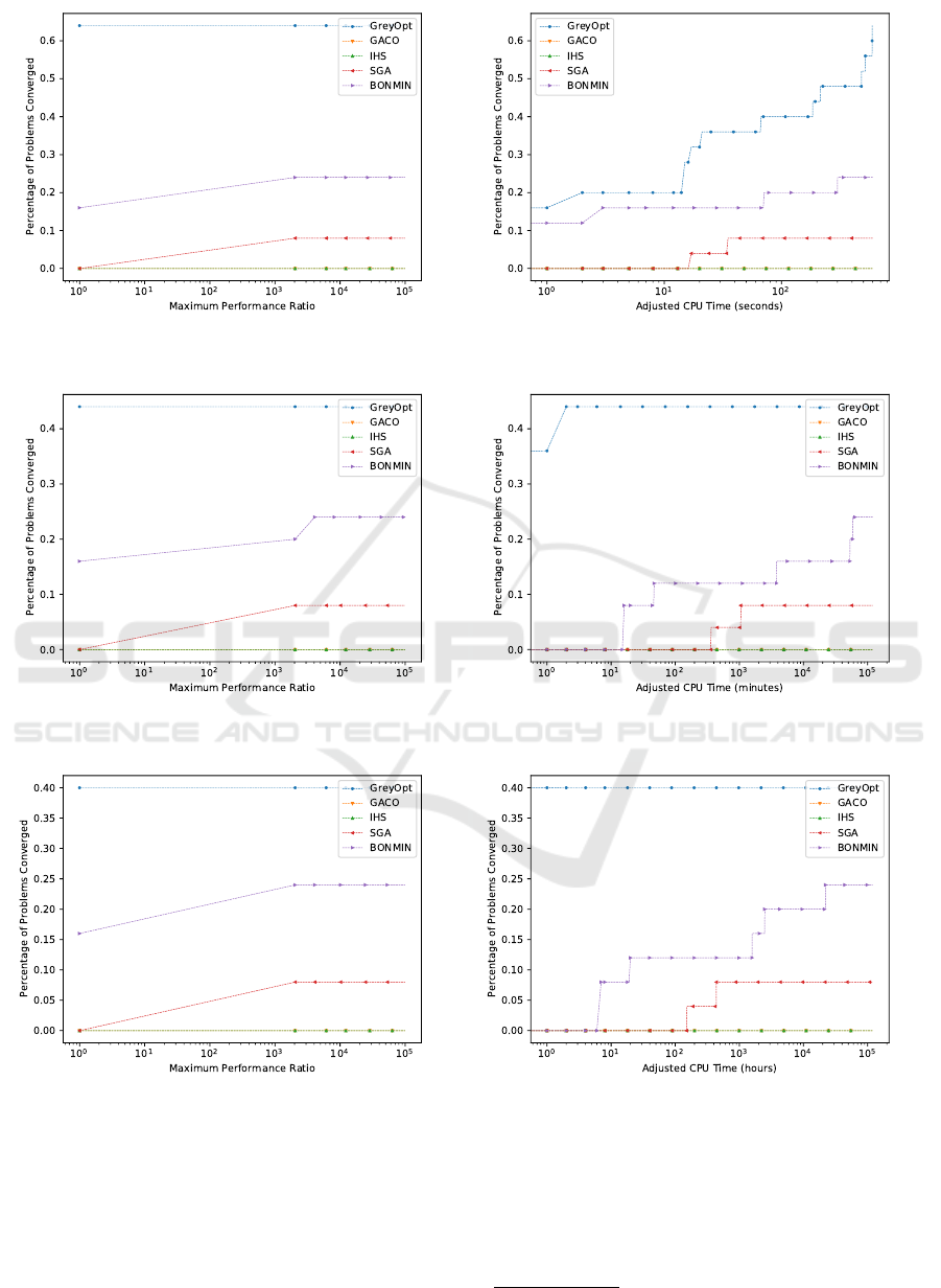
(a) Performance Profile
BBT = 0 seconds (per call).
(b) Data Profile
BBT = 0 seconds (per call).
(c) Performance Profile
BBT = 1 second (per call).
(d) Data Profile
BBT = 1 second (per call).
(e) Performance Profile
BBT = 10 seconds (per call).
(f) Data Profile
BBT = 10 seconds (per call).
Figure 2: Performance and data profiles using the median of multiple runs of each algorithm for different levels of black-box
function computation times (BBT).
rithms in Pygmo2 that support mixed-integer opti-
mization. We were unable to find any available imple-
mentation of a grey-box optimization algorithm that
supports MICGB problems. Although an open-source
implementation in MATLAB of DEFT-FUNNEL is
available on GitHub
6
, it does not support MICGB
6
https://github.com/phrsampaio/deft-funnel
ICORES 2021 - 10th International Conference on Operations Research and Enterprise Systems
108

imp ort g r e y o p t . n u m e r i c s a s n
d ef t r i g x m o d e l ( in pu t , o p t i o n s ={} ) :
b b t = o p t i o n s . g e t ( ” b b t ” , None )
x2 = i n p u t [ ” x2 ” ]
x3 = i n p u t [ ” x3 ” ]
r et u r n {
” o b j ” : n . c a l l ( lambda x2 : x2 ∗ x2 , x2 , b b t = b b t )
+ x3 ∗ x3 ,
” c o n s t r a i n t s ” : {
” e 2 ” : x2 − n . c a l l ( lambda x2 , x3 : n . s i n (
2 . 0 ∗ x2 + 3 . 0 ∗ x3 ) , x2 , x3 , b b t = b b t )
− n . co s ( 3 . 0 ∗ x2 − 5 . 0 ∗ x3 ) == 0 . 0 ,
” e 3 ” : x3 − n . c a l l ( lambda x2 , x3 : n . s i n (
x2 − 2 . 0 ∗ x3 ) , x2 , x3 , b b t = b b t )
+ n . c o s ( x2 + 3 . 0 ∗ x3 ) == 0 . 0
}
}
d ef t r i g x ( o p t i o n s ={}) :
o u t p u t = t r i g x m o d e l ( {
” x2 ” : n . v a r i a b l e ( name=” x2 ” , v a l u e =None ,
bo un ds =[ f l o a t ( ”−i n f ” ) , f l o a t ( ” i n f ” ) ] ) ,
” x3 ” : n . v a r i a b l e ( name=” x3 ” , v a l u e =None ,
bo un ds =[ f l o a t ( ”−i n f ” ) , f l o a t ( ” i n f ” ) ] )
} , o p t i o n s )
r et u r n n . p ro b le m ( name=” t r i g x ” ,
o b j e c t i v e s = [ o u t p u t [ ” o b j ” ] ] ,
c o n s t r a i n t s = o u t p u t [ ” c o n s t r a i n t s ” ] ,
o p t i o n s = o p t i o n s )
Figure 3: Python code for MIGCB problem derived from
the trigx problem of MINLPLib.
problems.
In addition to these derivative-free algorithms, we
also report results for BONMIN, a mixed-integer con-
vex nonlinear solver, where the first order deriva-
tives are computed using a combination of automatic
differentiation for analytical expressions and finite-
differences for embedded black-box function calls.
All algorithms were configured with their default op-
tions selected.
4.3 Experimental Setup
The prototype of GREYOPT used for this study has
been implemented in Python and depends on six
open-source Python packages: (1) CasADi
7
v3.5.5,
(2) NumPy
8
v1.19.4, (3) PyInterval
9
v1.2.0, (4)
Scikit-Learn
10
v0.23.2, (5) SciPy
11
v1.5.4, and (5)
7
URL: https://github.com/casadi/casadi
8
URL: https://github.com/numpy/numpy
9
URL: https://github.com/taschini/pyinterval
10
URL: https://github.com/scikit-learn/scikit-learn
11
URL: https://github.com/scipy/scipy
SortedContainers
12
v2.3.0. CasADi (Andersson et al.,
2019) is a software framework for nonlinear opti-
mization and optimal control that GREYOPT uses for
symbolic computation, automatic differentiation, and
interfaces for derivative-based optimization solvers.
Specifically, GREYOPT uses the convex nonlinear
solvers IPOPT (Biegler and Zavala, 2009) and BON-
MIN (Bonami et al., 2008) for the optimization of the
surrogate problems. GREYOPT uses PyInterval (Tas-
chini, 2008) for computing the intervals of analytical
expressions. GREYOPT uses Scikit-Learn (Pedregosa
et al., 2011) for polynomial and Gaussian process re-
gression.
We extend each black-box function to accept a pa-
rameter, BBT, that controls how much additional CPU
time, in seconds, to consume for each call to that func-
tion. Instead of wasting CPU cycles for the duration
of BBT, in this study the actual CPU time that is mea-
sured and reported is adjusted by c × BBT, where c
is the total number of calls to black-box functions.
This can be used to make an otherwise inexpensive
black-box function appear more expensive to both the
algorithm and the experimental study, without having
to modify the structure of the problem. In this study,
three different levels of BBT are considered: 0 sec-
onds, 1 second, and 10 seconds.
All experiments were run on ARGO-1, a research
computing cluster provided by the Office of Research
Computing
13
at George Mason University. We adopt
the same CPU time budget as used by Rios and
Sahinidis (2009), where each algorithm is allocated
a budget of 10 CPU minutes to optimize each prob-
lem. Although the measured and reported CPU time
is adjusted by the BBT parameter, we do not adjust the
CPU time budget. Each trial of this study involved
running an algorithm on a problem for the duration of
the CPU time budget and recording the convergence
trace of the objective value of the best feasible point
found over a BBT-adjusted CPU time horizon. If a
feasible point has not yet been found, a value of ∞ is
assumed for the objective.
While the problems considered in this study are
all deterministic, some of the algorithms tested are
stochastic, where multiple runs of the same algorithm
on the same problem with the same starting point can
return different results. To account for this, we con-
ducted 15 trials for each experiment that consumed
over 312 hours of CPU time on the cluster. We report
the median objective value, which is robust to outliers,
instead of the mean since we use a value of ∞ for the
objective of infeasible points.
12
URL: https://github.com/grantjenks/python-
sortedcontainers
13
URL: https://orc.gmu.edu
Mixed-Integer Constrained Grey-Box Optimization based on Dynamic Surrogate Models and Approximated Interval Analysis
109

4.4 Evaluation Methodology
The evaluation methodology of this study is based on
the performance profile of Dolan and Mor
´
e (2002)
and the data profile of Mor
´
e and Wild (2009). In this
section we denote the set of algorithms listed in Sec-
tion 4.2 by A , and the set of problems listed in Table 1
by P . Because none of the algorithms for MICGB op-
timization tested in this study are globally convergent
to a global optima in finite time, we use the following
test of relative convergence for an algorithm a ∈ A on
a problem p ∈ P :
f
∗
− f
a
>= (1 − τ)( f
∗
− f
∗
) (10)
where f
∗
is the worst (i.e. highest) objective value
among the set containing the first feasible point found,
if any, by each algorithm a ∈ A for problem p, where
f
∗
is the best (i.e. lowest) objective value among the
feasible points found by any algorithm a ∈ A on prob-
lem p, where f
a
is the objective value of the best point
found, feasible or otherwise, by algorithm a on prob-
lem p, and where τ is the tolerance parameter. We
use the same tolerance used by Costa and Nannicini
(2018) of τ , 10
−3
.
The performance ratio r
p,a
for a problem p ∈ P
and an algorithm a ∈ A is defined by Dolan and Mor
´
e
(2002) as:
r
p,a
,
t
p,a
min{t
p,a
: a ∈ A}
(11)
where t is the performance measure of interest. In
this study, we define t
p,a
as the minimum median
BBT-adjusted CPU time, in seconds, that algorithm a
needed to converge for problem p, based on the con-
vergence test in Equation 10. If algorithm a failed to
converge for problem p, then we assign t
p,a
the value
of ∞.
The performance profile of Dolan and Mor
´
e
(2002) is defined in this study as follows:
ρ
a
(x) ,
|{p ∈ P : r
p,a
≤ x}|
|P |
(12)
where ρ
a
(x) for algorithm a is the percentage of prob-
lems P where the performance ratio r
p,a
is less than
or equal to x. The lowest value that parameter x can
be is equal to the best possible performance ratio (i.e.
1).
Finally, the data profile of Mor
´
e and Wild (2009)
is defined in this study as follows:
d
a
(x) ,
|{p ∈ P : t
p,a
≤ x}|
|P |
(13)
where d
a
(x) is the percentage of problems P that al-
gorithm a converges for within x BBT-adjusted CPU
seconds.
4.5 Results
The results of this study are shown in Figure 2, where
plots of the data and performance profile for each BBT
level tested are provided. Starting with the perfor-
mance profile for BBT = 0 seconds (per call), GREY-
OPT converges on over 60% of the problems tested
when the performance ratio is equal to 1 (i.e. the
best possible case). The data profile for BBT = 0 sec-
onds (per call) shows that the number of problems
that GREYOPT converges on steadily increases over
the CPU time horizon. Moving on to the performance
profile for BBT = 1 second (per call), the percentage of
problems that GREYOPT converges on drops to about
43%, but is still considerably more than the next best
algorithm, multi-start BONMIN. To account for the
large increase in computational effort required by the
other solvers, the data profile for BBT = 1 second (per
call) switches the units of the horizontal axis from ad-
justed CPU seconds to adjusted CPU minutes. Simi-
larly is the case for both the performance and data pro-
file for BBT = 10 seconds (per call), where the units of
the horizontal axis jumps from adjusted CPU minutes
to adjusted CPU hours. Both the performance pro-
file and data profile show that GREYOPT significantly
outperforms all of other algorithms evaluated in this
study, even outperforming the multi-start BONMIN
algorithm when the black-box functions are cheap.
5 CONCLUSIONS
The GREYOPT algorithmic framework has been pro-
posed for the heuristic global optimization of MICGB
problems. We have shown how the partially ana-
lytical structure of such problems can be leveraged
to guide the exploration of the search space using
dynamically constructed surrogate problems and ap-
proximations of the intervals of grey-box objective
and constraint functions. We have conducted an
experimental study of GREYOPT’s performance on
a set of 25 MICGB optimization problems derived
from MINLPLib where the ratio of black-box func-
tion evaluations to analytical expressions is small.
The results of the study show that GREYOPT signifi-
cantly outperforms the three derivative-free optimiza-
tion algorithms evaluated on these problems, as well
as a random restart version of the open-source convex
nonlinear optimization solver BONMIN.
The development of GREYOPT is an ongoing ef-
fort. Possible directions for future work include: (1)
extending GREYOPT to support multi-objective op-
timization, (2) direct support for the optimization of
problems containing calls to noisy black-box func-
ICORES 2021 - 10th International Conference on Operations Research and Enterprise Systems
110

tions, and (3) incorporating meta-optimization tech-
niques for the automatic, problem-specific configura-
tion of GREYOPT’s parameters.
REFERENCES
Andersson, J. A. E., Gillis, J., Horn, G., Rawlings, J. B.,
and Diehl, M. (2019). CasADi: a software framework
for nonlinear optimization and optimal control. Math-
ematical Programming Computation, 11(1):1–36.
Androulakis, I. P., Maranas, C. D., and Floudas, C. A.
(1995). αBB: A global optimization method for gen-
eral constrained nonconvex problems. Journal of
Global Optimization, 7(4):337–363.
Biegler, L. T. and Zavala, V. M. (2009). Large-scale nonlin-
ear programming using ipopt: An integrating frame-
work for enterprise-wide dynamic optimization. Com-
puters & Chemical Engineering, 33(3):575–582.
Biscani, F. and Izzo, D. (2020). A parallel global multiob-
jective framework for optimization: pagmo. Journal
of Open Source Software, 5(53):2338.
Bonami, P., Biegler, L. T., Conn, A. R., Cornu
´
ejols, G.,
Grossmann, I. E., Laird, C. D., Lee, J., Lodi, A., Mar-
got, F., Sawaya, N., and W
¨
achter, A. (2008). An algo-
rithmic framework for convex mixed integer nonlinear
programs. Discrete Optimization, 5(2):186 – 204.
Boukouvala, F. and Floudas, C. A. (2017). ARGONAUT:
AlgoRithms for Global Optimization of coNstrAined
grey-box compUTational problems. Optimization Let-
ters, 11(5):895–913.
Brodsky, A., Nachawati, M. O., Krishnamoorthy, M., Bern-
stein, W. Z., and Menasc
´
e, D. A. (2019). Factory op-
tima: a web-based system for composition and anal-
ysis of manufacturing service networks based on a
reusable model repository. International journal of
computer integrated manufacturing, 32(3):206–224.
Brodsky, A. and Wang, X. S. (2008). Decision-Guidance
Management Systems (DGMS): Seamless Integration
of Data Acquisition, Learning, Prediction and Opti-
mization. In Proceedings of the Proceedings of the
41st Annual Hawaii International Conference on Sys-
tem Sciences.
Charnes, A. and Cooper, W. W. (1959). Chance-
Constrained Programming. Management Science,
6(1):73–79.
Costa, A. and Nannicini, G. (2018). RBFOpt: an open-
source library for black-box optimization with costly
function evaluations. Mathematical Programming
Computation, 10(4):597–629.
Dolan, E. D. and Mor
´
e, J. J. (2002). Benchmarking opti-
mization software with performance profiles. Mathe-
matical programming, 91(2):201–213.
Farmani, R. and Wright, J. A. (2003). Self-adaptive fitness
formulation for constrained optimization. IEEE trans-
actions on evolutionary computation, 7(5):445–455.
Gilboa, E., Saatc¸i, Y., and Cunningham, J. (2013). Scaling
multidimensional gaussian processes using projected
additive approximations. In International Conference
on Machine Learning, pages 454–461.
Hansen, N., Auger, A., Ros, R., Finck, S., and Po
ˇ
s
´
ık, P.
(2010). Comparing Results of 31 Algorithms from
the Black-Box Optimization Benchmarking BBOB-
2009. In Proceedings of the 12th Annual Conference
Companion on Genetic and Evolutionary Computa-
tion, pages 1689–1696.
Jones, D. R., Schonlau, M., and Welch, W. J. (1998).
Efficient Global Optimization of Expensive Black-
Box Functions. Journal of Global Optimization,
13(4):455–492.
Mahdavi, M., Fesanghary, M., and Damangir, E. (2007). An
improved harmony search algorithm for solving opti-
mization problems. Applied Mathematics and Com-
putation, 188(2):1567–1579.
Mazumdar, A., Chugh, T., Miettinen, K., and L
´
opez-Ib
´
a
˜
nez,
M. (2019). On Dealing with Uncertainties from
Kriging Models in Offline Data-Driven Evolution-
ary Multiobjective Optimization. Evolutionary Multi-
Criterion Optimization, pages 463–474. ISBN: 978-
3-030-12598-1 Place: Cham Publisher: Springer In-
ternational Publishing.
McCormick, G. P. (1976). Computability of global so-
lutions to factorable nonconvex programs: Part I
— Convex underestimating problems. Mathematical
Programming, 10(1):147–175.
Misener, R. and Floudas, C. A. (2014). ANTIGONE: Algo-
rithms for coNTinuous / Integer Global Optimization
of Nonlinear Equations. Journal of Global Optimiza-
tion, 59(2):503–526.
Moore, R. E. (1966). Interval analysis. Prentice-Hall series
in automatic computation. Prentice-Hall, Englewood
Cliffs, NJ.
Mor
´
e, J. J. and Wild, S. M. (2009). Benchmarking
Derivative-Free Optimization Algorithms. SIAM
Journal on Optimization, 20(1):172–191. Publisher:
Society for Industrial and Applied Mathematics.
Nachawati, M. O., Brodsky, A., and Luo, J. (2017). Unity
Decision Guidance Management System: Analytics
Engine and Reusable Model Repository. In Proceed-
ings of the 19th International Conference on Enter-
prise Information Systems - Volume 3: ICEIS,, pages
312–323. SciTePress.
Oliveto, P. S., He, J., and Yao, X. (2007). Time complex-
ity of evolutionary algorithms for combinatorial opti-
mization: A decade of results. International Journal
of Automation and Computing, 4(3):281–293.
Pedregosa, F., Varoquaux, G., Gramfort, A., Michel, V.,
Thirion, B., Grisel, O., Blondel, M., Prettenhofer, P.,
Weiss, R., Dubourg, V., et al. (2011). Scikit-learn:
Machine learning in python. the Journal of machine
Learning research, 12:2825–2830.
Pint
´
er, J. D. (1997). LGO — A Program System for Contin-
uous and Lipschitz Global Optimization. In Bomze,
I. M., Csendes, T., Horst, R., and Pardalos, P. M.,
editors, Developments in Global Optimization, pages
183–197. Springer US, Boston, MA.
Rios, L. and Sahinidis, N. (2009). Derivative-free optimiza-
tion: A review of algorithms and comparison of soft-
Mixed-Integer Constrained Grey-Box Optimization based on Dynamic Surrogate Models and Approximated Interval Analysis
111

ware implementations. Journal of Global Optimiza-
tion, 56.
Sampaio, P. R. (2019). DEFT-FUNNEL: an open-
source global optimization solver for constrained
grey-box and black-box problems. arXiv preprint
arXiv:1912.12637.
Schl
¨
uter, M., Egea, J. A., and Banga, J. R. (2009). Ex-
tended ant colony optimization for non-convex mixed
integer nonlinear programming. Computers & Oper-
ations Research, 36(7):2217–2229.
Talbi, E.-G. (2013). A Unified Taxonomy of Hybrid Meta-
heuristics with Mathematical Programming, Con-
straint Programming and Machine Learning. In Talbi,
E.-G., editor, Hybrid Metaheuristics, pages 3–76.
Springer Berlin Heidelberg, Berlin, Heidelberg.
Taschini, S. (2008). Interval arithmetic: Python implemen-
tation and applications. In Proceedings of the 7th
Python in Science Conference, Pasadena, CA USA,
pages 16–21.
W
¨
achter, A. and Biegler, L. T. (2006). On the implemen-
tation of an interior-point filter line-search algorithm
for large-scale nonlinear programming. Mathematical
Programming, 106(1):25–57.
Wengert, R. E. (1964). A simple automatic derivative
evaluation program. Communications of the ACM,
7(8):463–464.
APPENDIX
Tables 1 lists the MICGB problems tested in the ex-
perimental study presented in Section 4. For each
problem, we list its name, which corresponds to the
original problem from MINLPLib, the number of
variables, and the number of constraints.
Table 1: MICGB problems derived from MINLPLib.
Problem Variables Constraints
cvxnonsep psig20r 42 22
eniplac 141 189
ex1266a 48 53
ex14 2 3 6 9
ex14 2 5 4 5
ex8 4 8 bnd 42 30
ex8 5 3 5 4
feedtray2 88 284
glider100 1315 1209
inscribedsquare01 8 8
inscribedsquare02 8 8
kall circlesrectangles c1r12 49 52
kall circlesrectangles c6r1 184 192
nous2 50 43
pooling foulds2pq 36 34
sfacloc1
2 90 199 348
st e03 10 7
super3t 1056 1343
syn30h 228 345
wastepaper5 104 46
wastewater05m2 133 151
wastewater13m1 382 83
waterno2 01 166 204
waterund01 40 38
waterund18 60 64
ICORES 2021 - 10th International Conference on Operations Research and Enterprise Systems
112