Processing Attribute Profiles as Scale-series for Remote Sensing Image
Classification
Melike Ilteralp
1 a
and Erchan Aptoula
2 b
1
Department of Computer Engineering, Gebze Technical University, Kocaeli, Turkey
2
Institute of Information Technologies, Gebze Technical University, Kocaeli, Turkey
Keywords:
Attribute Profiles, Hyperspectral Images, Supervised Classification, Long Short-term Memory Network.
Abstract:
Attribute profiles (APs) are among the most prominent “shallow” spatial-spectral pixel description methods,
providing multi-scale, flexible and efficient pixel descriptions, even with modest amounts of training data. In
this paper, we investigate their collaboration with long short-term memory networks (LSTMs). Our hypothesis
is that a profile can be viewed as a “scale-series” and LSTMs can exploit their sequential nature, akin to
temporal series. Plus, feeding a deep network with input of already strong descriptive potential (such as APs)
can help them produce advanced features more efficiently w.r.t. training from scratch. Moreover, contrary to
the state-of-the-art, we report the results of experiments conducted with non-overlapping training and testing
sets, highlighting a significant boost of performance through the combined use of APs with LSTMs.
1 INTRODUCTION
Pixel-level classification with the end goal of land
use/cover mapping constitutes the basis of several
remote sensing applications. Despite numerous re-
ported pixel description methods, it represents a long-
standing challenge due to constant sensor technology
advances. Ever-increasing spatial, spectral and tem-
poral remote sensing image resolutions have ampli-
fied the need for efficient and effective spatial-spectral
pixel description and classification approaches (Land-
grebe, 2003).
Deep learning is known for its state-of-the-art
performance across many domains, including remote
sensing (Audebert et al., 2019). However, its perfor-
mance is tightly bounded by its need for a large num-
ber of labeled samples as well as for high label pre-
cision. In addition, labeled remote sensing datasets
are relatively scarce w.r.t. computer vision, since gen-
erating them is an arduous and expensive task. Con-
sequently, it is not surprising that shallow approaches
are still widely employed, as in the recent IEEE GRSS
Data Fusion Contest (Yokoya et al., 2020).
At the front of “shallow” descriptors, Morpholog-
ical Attribute Profiles (APs) stand out as a prominent
approach, even with modest amounts of training data.
a
https://orcid.org/0000-0003-2685-914X
b
https://orcid.org/0000-0001-6168-2883
By exploiting the hierarchical tree-based representa-
tions of an input image, they produce multi-scale, ef-
ficient object-based pixel descriptions, w.r.t. arbitrar-
ily chosen criteria (Dalla Mura et al., 2010b). They
have been studied extensively in the past decade, in
terms of alternative tree representations (Bosilj et al.,
2017; Cavallaro et al., 2016), threshold selection tech-
niques (Bhardwaj et al., 2019; Derbashi and Aptoula,
2020), pre-processing (Dalla Mura et al., 2011) and
post-processing extensions (Pham et al., 2018). Nev-
ertheless, APs have their inconveniences too, as they
possess notoriously difficult to set parameters such as
thresholds and attributes.
An in-between approach to shallow and deep pixel
description has appeared as their combination in an
effort to harness the advantages of both strategies. It
consists in providing as input to relatively small deep
networks, easy to calculate shallow features; exam-
ples include the combination of Gabor filtered (Chen
et al., 2017) and attribute filtered images with con-
volutional neural networks (CNNs) (Aptoula et al.,
2016). The underlying motivation is to avoid training
from scratch (and hence circumvent the need for large
training sets), by starting from mid-level features and
to produce more advanced outputs through the ability
of deep networks.
In this paper, we explore further the aforemen-
tioned pixel description paradigm of combining shal-
low and deep strategies. More specifically, since a
558
Ilteralp, M. and Aptoula, E.
Processing Attribute Profiles as Scale-series for Remote Sensing Image Classification.
DOI: 10.5220/0010350005580565
In Proceedings of the 16th International Joint Conference on Computer Vision, Imaging and Computer Graphics Theory and Applications (VISIGRAPP 2021) - Volume 4: VISAPP, pages
558-565
ISBN: 978-989-758-488-6
Copyright
c
 2021 by SCITEPRESS – Science and Technology Publications, Lda. All rights reserved

pixel’s values across an attribute profile constitute a
numerical sequence across scales, it can be consid-
ered as a “scale series”. Consequently, we have se-
lected a long short-term memory (LSTM) network in
order to exploit its sequential nature, akin to temporal
series analysis (Hochreiter and Schmidhuber, 1997).
Our second contribution addresses a validation
mis-conduct encountered very often in the AP related
literature, where a single tree representation is calcu-
lated from the entire scene of the ground truth. As a
result, the same tree encodes the pixels of both train-
ing and testing sets, leading very possibly to pixels of
the same connected components used both for model
development and validation. Evidently, this can lead
to unrealistically high classification performances and
deceivingly high generalization impressions (Aude-
bert et al., 2019).
To avoid this, we have conducted experiments
with two real-world datasets, where non-overlapping
training and test subsets are used, or in other words,
distinct tree representations are calculated for train-
ing and testing. The results confirm this performance
discrepancy, while the proposed combination of APs
with LSTMs achieves significantly higher generaliza-
tion performance.
2 PROPOSED APPROACH
This section will first recall the basics of APs, hierar-
chical tree representations and LSTMs, and then elab-
orate on the proposed approach for pixel description.
2.1 Attribute Profiles
APs are efficient, multiscale image descriptors that
have been introduced in order to overcome the struc-
turing element related limitations of the older mor-
phological profiles (Dalla Mura et al., 2010b). APs
are based on attribute filters (AFs) which are morpho-
logical connected filters that either preserve or remove
connected components (CC) of grayscale images via
checking whether that CC satisfies a binary predicate.
The predicate is typically a comparison of a CC at-
tribute (e.g. area, elongation, etc) against a numerical
threshold value. APs consist of a series of images that
are generated via stacking the outputs of AFs using
progressively increasing threshold values.
More formally, let f : D → Z be a grayscale im-
age where D ⊆ Z
2
. Let T be a binary predicate and
{κ
i
}
1≤i≤L
a set of L thresholds. Let γ
κ
i
and φ
κ
i
be
the morphological thinning and thickening filters with
threshold κ
i
. The AP of f is obtained as follows:
AP( f ) = {φ
κ
L
( f ), φ
κ
L−1
( f ), . . . , φ
κ
1
( f ), f ,
γ
κ
1
( f ), . . . , γ
κ
L−1
( f ), γ
κ
L
( f )}
(1)
Extended attribute profiles (EAPs) (Dalla Mura
et al., 2010a) represent the extension of APs to hy-
perspectral images. EAPs are generated via applying
a dimensionality reduction technique to a hyperspec-
tral image f
f
f and then stacking the calculated AP of
each remaining band:
EAP( f
f
f ) = {AP(band
1
), AP(band
2
), . . . , AP(band
n
)}
(2)
In both cases (AP and EAP), individual pixels are
described with the sequence of values they acquire
across the filtered images. In addition, the spatial de-
tail level associated with each value in this sequence
decreases as the employed threshold value increases.
Hence, an AP can be considered as a pixel-level scale-
series.
2.2 Hierarchical Tree Representation
Even though AF have been known for a long time
(Breen et al., 1996), the computational complexity
of CC calculation has hindered their widespread use.
This changed with the manifestation of hierarchical
tree-based image representations (Salembier et al.,
1998), where CCs are encoded as tree-nodes. Conse-
quently, it becomes possible to efficiently manipulate
entire CCs and perform object based filtering through
mere tree pruning operations.
In more detail, the hierarchical representation of
an image is formed via stacking the union of image
regions at different scales (Bosilj et al., 2018). The
tree structure stands forward as a prominent hierar-
chical image representation since each tree node cor-
responds to an image region and the parent-child rela-
tion between the tree nodes indicates the inclusion re-
lation of the image regions of different scales. In this
tree structure, which is called a component tree, the
leaf nodes correspond to the finest regions of the im-
age and the region covered by a node grows as moving
higher (towards the root node) in the tree where the
root node corresponds to the whole image. There are
two types of component tree categories, the inclusion
trees and the partition trees where the distinction be-
tween them is how the hierarchy is built (Bosilj et al.,
2018).
The inclusion trees (such max/min trees) consist
of the partial partition of the image and the leaf nodes
correspond to the small regions of the image such as
local minima or maxima. The new nodes are formed
via including the same intensity pixels (flat zones) to
the leaf nodes and this inclusion of pixels forms the
Processing Attribute Profiles as Scale-series for Remote Sensing Image Classification
559

...
FC1
(ReLU)
LSTM1
(32cells)
LSTM3
(32cells)
LSTM2
(32cells)
FC2 Softmax
Inputimage
(hyperspectralor
panchromatic)
PCAfor
hyperspectral
images
rPrincipal
Components
AP
calculation
Pixelptobe
described
AP
1,1
AP
1,L
PC
1
...
AP
r,1
AP
r,L
PC
r
...
...
PC
1
PC
r
...
...
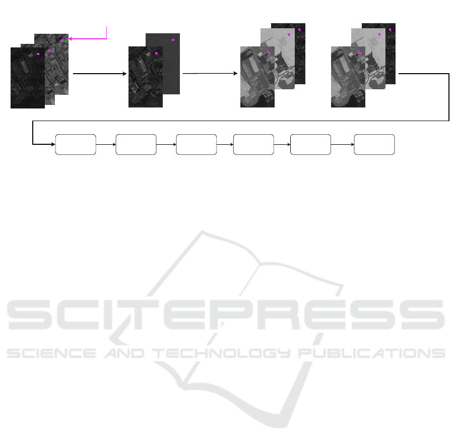
Figure 1: Outline of our pixel description strategy and the architecture of the model where PCA, PC, FC and ReLU, denote
principal component analysis, principal component image, fully connected layer and rectified linear unit respectively.
parent-child relationship between them. Inclusion of
the pixels to the nodes and hence the formation of
the new nodes continues until the root node where the
root node corresponds to the whole image.
The partition trees (such as α-trees, binary parti-
tion trees) comprise the full partition of the image and
the leaf nodes containing the finest image regions are
merged as moving higher in the tree where the root
node corresponds to the whole image (Bosilj et al.,
2017). The partition at any level of the partition tree
represents the whole image.
2.3 Long Short-Term Memory
Networks
LSTMs are known to achieve state-of-art perfor-
mance with various sequential data tasks (Hochre-
iter and Schmidhuber, 1997; Ma and Hovy, 2016;
Søgaard and Goldberg, 2016). A LSTM is a spe-
cialized recurrent neural network (RNN) architecture
that is designed to process sequential data. RNN uses
the information of previous events to make inference
about the future event along with the current one by
retaining the past knowledge with its chain-like struc-
ture. However, RNNs suffer from the inability to learn
long-term dependencies between the events with large
time gaps, due to vanishing gradients. LSTMs have
been in fact introduced to address specifically this is-
sue.
In more detail, a LSTM cell receives a sequential
data sample x
t
∈ R
n
, a hidden state h
t−1
and the cell
state C
t−1
of the previous cell as input at time t and
calculates the current cell state C
t
and hidden state
h
t
with forget, input and output gates within it. The
forget gate f
t
calculates how much of the previous and
current information will be kept. The input gate i
t
calculates which values are important for updating the
cell state C
t
. The output gate o
t
calculates the current
hidden state h
t
. Formally, the output of a LSTM cell
at time t is calculated as follows:
f
t
= σ(W
f
· x
t
+U
f
· h
t−1
+ b
f
)
i
t
= σ(W
i
· x
t
+U
i
· h
t−1
+ b
i
)
o
t
= σ(W
o
· x
t
+U
o
· h
t−1
+ b
o
)
˜
C
t
= tanh(W
c
· x
t
+U
c
· h
t−1
+ b
c
)
C
t
= f
t
◦C
t−1
+ i
t
◦
˜
C
t
h
t
= o
t
◦tanh(C
t
)
(3)
where σ denotes the sigmoid function, · denotes the
matrix multiplication, ◦ denotes the dot product, W
∗
and U
∗
are weight matrices and b
∗
represent the bias
terms specific to the gates or cell state (Hochreiter and
Schmidhuber, 1997).
2.4 APs as Input to LSTMs
As explained in the previous section, an AP based
pixel feature vector constitutes a numerical sequence.
Each sequence element describes the pixel in terms of
an arbitrary pre-selected attribute (e.g. area) of the CC
containing it, at a certain spatial scale. And the scale
varies depending on the used threshold. Furthermore,
the values across an AP have no particular reason for
being independent of each other since they are gener-
ated via filtering the same input image. Therefore, a
neural model that can capture the eventual dependen-
cies within this scale series can potentially contribute
to classification performance.
However, convolutional neural networks don’t
treat data as a sequence and therefore, cannot exploit
“past” information. LSTMs on the other hand, stand
out as prominent DL architectures that can receive se-
quential data as input and capture eventual dependen-
cies within it.
VISAPP 2021 - 16th International Conference on Computer Vision Theory and Applications
560

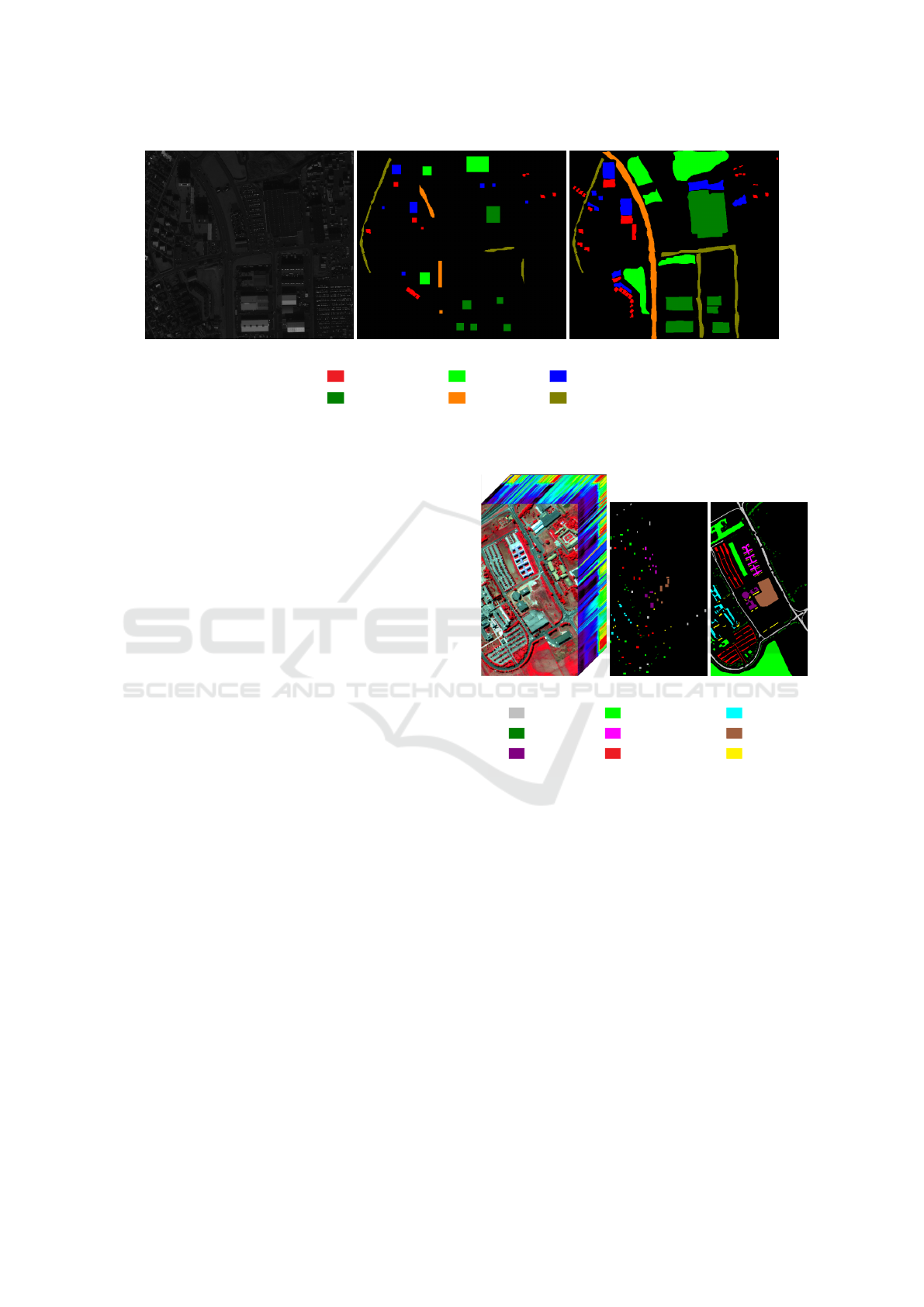
(a) Reykjavik Dataset
(b) Train Set
(c) Ground truth
Residential1:
Commercial4:
Soil2:
Highway5:
Shadow3:
Road6:
(d) Class labels
Figure 2: The Reykjavik dataset, training set and ground truth, as often encountered in the state-of-the-art.
Moreover, the combination of APs with deep
learning (DL) techniques can also help the latter by al-
leviating their need for a large amount of labeled data,
since APs constitute mid-level features and can thus
ease training by not forcing it to start from scratch
(Aptoula et al., 2016; Chen et al., 2017).
To achieve our goal, we adapted the LSTM model
of (Chevalier, 2016) which predicts the labels of se-
quences in a many-to-one manner that is similar to
our problem where each sequence of pixel descrip-
tion has a label. The proposed architecture consists
of 3 LSTM layers where each of them has 32 hidden
units. The choice of architectural hyperparameters is
detailed in Section 3.2.
The network architecture is not tuned for any one
dataset/tree representation since it’s intended for gen-
eral use. The outline of the proposed pixel description
strategy and the classification model is shown in Fig-
ure 1.
3 EXPERIMENTS
The aim of the experiments performed in this sec-
tion is to test our hypothesis that the combination of
APs, as mid-level features, with LSTMs yields supe-
rior generalization performance through the exploita-
tion of their sequential nature as scale-series.
3.1 Datasets
The experiments have been conducted on two real re-
mote sensing datasets, one being hyperspectral and
the other being a panchromatic dataset, in order to
show that our approach works for both types. The
(a) Pavia University (b) Training Set (c) Ground Truth
Asphalt1:
Trees
Bitumen
4:
7:
Meadows2:
Metalsheets
Self-blocking
bricks
5:
8:
Gravel3:
Baresoil
Shadows
6:
9:
(d) Class labels
Figure 3: The Pavia University dataset, training set and
ground truth, as often encountered in the state-of-the-art.
first one is the Pavia University dataset (Figure 3), ac-
quired by the ROSIS-03 sensor over Pavia, Italy. It is
an urban area consisting of 103 spectral bands, rang-
ing from 0.43 µm to 0.86 µm with 9 classes. It depicts
an area of 610 × 340 pixels and the spatial resolution
is 1.3 meters. After applying PCA to the dataset, four
principal components have been found to account for
99% of the total variance.
The second one is the panchromatic Reykjavik
dataset (Figure 2) acquired from Reykjavik, Iceland
with the Ikonos satellite. It shows an area of 628
× 700 pixels with 1 meter spatial resolution and 6
classes.
As observed by (Audebert et al., 2019), using
the standard train and test splits that are encountered
Processing Attribute Profiles as Scale-series for Remote Sensing Image Classification
561

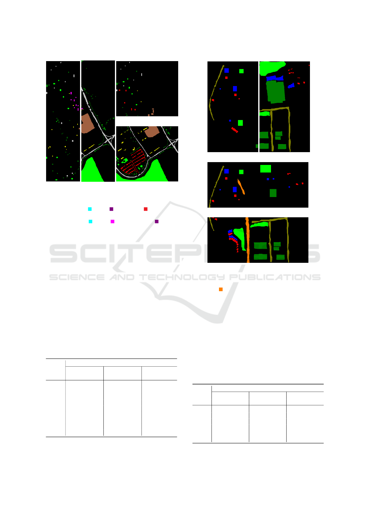
(a) Train I
(b) Test I
(c) Train II
(d) Test II
Figure 4: The Pavia University dataset train and test sets,
vertical split (a), (b) and horizontal split (c), (d). Note that
the samples of the gravel, bitumen and self-blocking
bricks classes are eliminated in the vertical split whereas
the samples of the gravel, metal sheets and bitumen
classes are eliminated in the horizontal split.
widely in the related state-of-the-art, one computes
a single tree, containing the nested connected com-
ponent hierarchy of both training and testing sam-
ples. Whereas in actual deployment conditions, the
classification models are expected to perform with
a distinct tree calculated from the scene to be clas-
sified. To overcome this issue, we generated non-
overlapping train/test subsets via splitting the ground
truth horizontally and vertically into two same-size
images. The top/left split is used as the train set and
the bottom/left split is used as the test set. The re-
sulting train and test sets depending on split type are
shown in Figures 4 and 5 for the Pavia University and
Table 1: The Pavia University dataset, number of class sam-
ples in the standard dataset and its horizontal and vertical
splits.
Labeled Samples per Split
Class Standard Horizontal Vertical
Id Train Test Train Test Train Test
1 548 6631 210 3499 392 3094
2 540 18649 240 13433 479 9035
3 392 2099 0 0 0 0
4 524 3064 214 1653 524 1176
5 265 1345 0 0 265 43
6 532 5029 372 3530 48 4634
7 375 1330 0 0 0 0
8 514 3682 225 1973 0 0
9 231 947 28 732 191 153
(a) Train I (b) Test I
(c) Train II
(d) Test II
Figure 5: The Reykjavik dataset train and test sets, vertical
split (a), (b) and horizontal split (c), (d). Note that the sam-
ples of the highway class are eliminated in the vertical
split.
the Reykjavik datasets respectively. Afterward, the
model is tested on both overlapping (Standard) and
non-overlapping (Horizontal and Vertical) train and
test subsets.
Some of the classes in the non-overlapping sub-
sets do not have a sufficient number of samples for
training or testing due to the split operation. To over-
come this situation, the ratio of the number of sam-
Table 2: The Reykjavik dataset, number of class samples in
the standard dataset and its horizontal and vertical splits.
Labeled Samples per Split
Class Standard Horizontal Vertical
Id Train Test Train Test Train Test
1 1863 6213 1195 1875 1446 669
2 6068 28144 4748 8885 2220 14419
3 2619 10610 2450 1278 2173 4078
4 5599 29768 2530 11893 450 27465
5 2489 12051 1300 5509 0 0
6 4103 11940 2147 9784 2828 8558
VISAPP 2021 - 16th International Conference on Computer Vision Theory and Applications
562

ples of a class w.r.t. the total number of samples in the
ground truth was enforced to be at least 0.1%. As a
result, the samples of the classes gravel, bitumen and
self-blocking bricks in the vertical split and the sam-
ples of the classes gravel, metal sheets and bitumen
in the horizontal split of the Pavia University dataset
have been eliminated. Likewise, samples of the high-
way class in the vertical split of the Reykjavik dataset
have been eliminated as well. The resulting num-
ber of samples per class depending on split type are
shown in Tables 1 and 2 for the Pavia University and
the Reykjavik datasets respectively.
3.2 Implementation Details
The area attribute has been selected in this study as a
geometric attribute for the sake of comparability rea-
sons with published studies (Dalla Mura et al., 2010b;
Bosilj et al., 2017; Cavallaro et al., 2016; Bhard-
waj et al., 2019; Derbashi and Aptoula, 2020; Dalla
Mura et al., 2011; Pham et al., 2018; Aptoula et al.,
2016). The CCs are calculated using two different
types of tree representations in the name of compre-
hensiveness. The first is a component (min-max) tree
from the family of inclusion trees and the other is an
α-tree from the family of partition trees. As far as
threshold selection is concerned, we used automat-
ically computed thresholds for the Pavia University
and Reykjavik datasets as recommended respectively
by (Ghamisi et al., 2014) and (Cavallaro et al., 2016):
λ
Pav
= {770, 1538, 2307, 3076, 3846, 4615, 5384, 6153,
6923, 7692, 8461, 9230, 10000, 10769}
λ
Rey
= {25, 100, 500, 1000, 5000, 10000, 20000,
50000, 100000, 150000}
(4)
The proposed approach has been compared
against two alternatives in order to better quantify its
effect:
• AP+RF (without LSTMs): APs are classified us-
ing a Random Forest (RF) classifier as is very of-
ten realized in the state-of-the-art.
• Spectral Signature + LSTM (without APs):
For the hyperspectral Pavia University dataset, a
LSTM was trained using its full 103-dimensional
spectral signature in order to observe the effect of
AP contribution w.r.t. to the plain use of LSTMs.
The RF classifier has been trained with 100 trees.
The same hyper-parameters have been used consis-
tently in the LSTM model across all experiments: a
learning rate of 0.0025, a batch size of 1500, and a
number of epochs of 9440 which are selected through
grid search. We fixed a seed=128 for reproducibil-
ity of the results. The time step of the LSTM model
is selected as 1 to be fair since the length of a pixel
description varies depending on the number of bands
of the dataset and the tree representation. The results
that have been obtained are shown in Table 3 and Ta-
ble 4.
3.3 Results & Discussion
The following observations can be made from the re-
sults of Table 3 and Table 4: when the standard (over-
lapping) train/test split is used, the RF classifier is
observed to achieve a superior performance w.r.t. the
LSTM model for both datasets, unless spectral signa-
tures are used. A possible explanation could be that
when using the standard train/test splits, many sam-
ples of the same connected components end up sep-
arated across the train and test sets. A deep network
is more prone to overfit w.r.t. RF, especially given the
relatively small dataset sizes.
On the contrary, when non-overlapping train/test
splits are used, the classification performance of RF
drops drastically and LSTM outperforms RF in all
non-overlapping image experiments for both datasets.
A possible explanation could be that when two pixels
of the same class from different sets (one from train
set and one from test set) are described by the APs cal-
culated from different trees, these descriptions will be
less similar to each other compared to the case where
both of them reside in the same tree. As LSTM treats
these descriptions as sequential data, not like indepen-
dent values as RF does, its performance is more ro-
bust than RF since it is able to exploit the sequential
nature of the information within the input sequence,
even though they are constructed using distinct trees.
This outcome also confirms the observations of (Au-
debert et al., 2019).
As verified by the results of the experiments in Ta-
ble 3 and Table 4, the benefit of combining APs with
LSTM is greater than the other approaches for the
classification performance on non-overlapping splits.
4 CONCLUSION
In this study, we explored the combination of APs
with LSTMs in an effort to exploit their sequen-
tial nature, that often goes under-exploited via the
widespread use of RF. For this purpose, we introduced
the collaboration of APs with LSTMs. We also inves-
tigated the usage of non-overlapping training and test-
ing sets and proposed a way to overcome their draw-
back on generalization performance.
Processing Attribute Profiles as Scale-series for Remote Sensing Image Classification
563

Table 3: Pixel classification performances in terms of the kappa statistic and F
1
-score × 100 for the Pavia University dataset
where AP+LSTM is the proposed approach.
Spectral Signature MinMax-tree α-tree
κ F
1
-score κ F
1
-score κ F
1
-score
Split RF LSTM RF LSTM AP+RF AP+LSTM AP+RF AP+LSTM AP+RF AP+LSTM AP+RF AP+LSTM
Standard 65.6 71.67 72.9 81.19 87.79 83.94 90.7 90.91 85.04 75.88 88.7 87.04
Vertical 36.83 44.28 52.5 62.91 17.22 49.7 34.5 65.56 15.69 33.49 26 55.06
Horizontal 33.57 42.07 35 68.64 25.08 59.89 39.3 71.49 45.61 60 58.4 74.53
Table 4: Pixel classification performances in terms of the kappa statistic and F
1
-score × 100 for the Reykjavik dataset where
AP+LSTM is the proposed approach.
MinMax-tree α-tree
κ F
1
-score κ F
1
-score
Split AP+RF AP+LSTM AP+RF AP+LSTM AP+RF AP+LSTM AP+RF AP+LSTM
Standard 76.46 58.26 82.5 57.07 71.56 65.61 77.8 65.34
Vertical 15.73 17.45 25.5 21.86 7.17 22.97 19 39.46
Horizontal 1.38 13.07 17.9 27.26 25.31 28.28 31.4 40.14
We tested our approach on two real remote sens-
ing datasets and APs have been calculated with two
different hierarchical tree representations. In all the
experiments where the training and testing sets don’t
overlap, we observed the collaboration of APs with
LSTM enabling a significant boost in classification
performance w.r.t. using AP or LSTMs alone.
In the future, we intend to address threshold-free
APs (Derbashi and Aptoula, 2020) via LSTMs capa-
ble of admitting varying length input. This will en-
able us to provide as input to the networks directly
the node sequences from the root node to the node
containing the pixel under study, eliminating the need
for cumbersome thresholds or filtering.
ACKNOWLEDGEMENTS
This study has been supported by TUBITAK under
Grant 118E258.
REFERENCES
Aptoula, E., Ozdemir, M. C., and Yanikoglu, B. (2016).
Deep learning with attribute profiles for hyperspectral
image classification. IEEE Geoscience and Remote
Sensing Letters, 13(12):1970–1974.
Audebert, N., Le Saux, B., and Lef
`
evre, S. (2019). Deep
learning for classification of hyperspectral data: A
comparative review. IEEE Geoscience and Remote
Sensing Magazine, 7(2):159–173.
Bhardwaj, K., Patra, S., and Bruzzone, L. (2019).
Threshold-free attribute profile for classification of
hyperspectral images. IEEE Transactions on Geo-
science and Remote Sensing, 57(10):7731–7742.
Bosilj, P., Damodaran, B., Aptoula, E., Dalla Mura, M., and
Lef
`
evre, S. (2017). Attribute profiles from partitioning
trees. In Mathematical Morphology and Its Applica-
tions to Signal and Image Processing, pages 381–392.
Springer International Publishing.
Bosilj, P., Kijak, E., and Lef
`
evre, S. (2018). Partition and in-
clusion hierarchies of images: A comprehensive sur-
vey. Journal of Imaging, 4(2):1–31.
Breen, E. J., , and Jones, R. (1996). Attribute openings,
thinnings, and granulometries. Computer Vision and
Image Understanding, 64(3):377–389.
Cavallaro, G., Dalla Mura, M., Benediktsson, J. A., and
Plaza, A. (2016). Remote sensing image classification
using attribute filters defined over the tree of shapes.
IEEE Transactions on Geoscience and Remote Sens-
ing, 54(7):3899–3911.
Chen, Y., Zhu, L., Ghamisi, P., Jia, X., Li, G., and
Tang, L. (2017). Hyperspectral images classifica-
tion with Gabor filtering and convolutional neural net-
work. IEEE Geoscience and Remote Sensing Letters,
14(12):2355–2359.
Chevalier, G. (2016). LSTMs for human activity
recognition. https://github.com/guillaume-chevalier/
LSTM-Human-Activity-Recognition, visited 2020-
11-12.
Dalla Mura, M., Benediktsson, J. A., Waske, B., and Bruz-
zone, L. (2010a). Extended profiles with morpho-
logical attribute filters for the analysis of hyperspec-
tral data. International Journal of Remote Sensing,
31(22):5975–5991.
Dalla Mura, M., Benediktsson, J. A., Waske, B., and
Bruzzone, L. (2010b). Morphological attribute pro-
files for the analysis of very high resolution images.
IEEE Transactions on Geoscience and Remote Sens-
ing, 48(10):3747–3762.
Dalla Mura, M., Villa, A., Benediktsson, J. A., Chanus-
sot, J., and Bruzzone, L. (2011). Classification of hy-
perspectral images by using extended morphological
attribute profiles and independent component analy-
sis. IEEE Geoscience and Remote Sensing Letters,
8(3):542–546.
Derbashi, U. and Aptoula, E. (2020). Attribute profiles
without thresholds through histogram based tree path
VISAPP 2021 - 16th International Conference on Computer Vision Theory and Applications
564

description. In 2020 Mediterranean and Middle-East
Geoscience and Remote Sensing Symposium, pages
29–32.
Ghamisi, P., Benediktsson, J. A., and Sveinsson, J. R.
(2014). Automatic spectral–spatial classification
framework based on attribute profiles and supervised
feature extraction. IEEE Transactions on Geoscience
and Remote Sensing, 52(9):5771–5782.
Hochreiter, S. and Schmidhuber, J. (1997). Long short-term
memory. Neural Computation, 9(8):1735–1780.
Landgrebe, D. A. (2003). Signal Theory Methods in Multi-
spectral Remote Sensing. Wiley, New York.
Ma, X. and Hovy, E. (2016). End-to-end sequence label-
ing via bi-directional LSTM-CNNs-CRF. In Proceed-
ings of the 54th Annual Meeting of the Association for
Computational Linguistics (Volume 1: Long Papers),
pages 1064–1074, Berlin, Germany.
Pham, M., Lef
`
evre, S., and Aptoula, E. (2018). Lo-
cal feature-based attribute profiles for optical remote
sensing image classification. IEEE Transactions on
Geoscience and Remote Sensing, 56(2):1199–1212.
Salembier, P., , Oliveras, A., and Garrido, L. (1998).
Antiextensive connected operators for image and se-
quence processing. IEEE Transactions on Image Pro-
cessing, 7(4):555–570.
Søgaard, A. and Goldberg, Y. (2016). Deep multi-task
learning with low level tasks supervised at lower lay-
ers. In Proceedings of the 54th Annual Meeting of the
Association for Computational Linguistics (Volume 2:
Short Papers), pages 231–235, Berlin, Germany.
Yokoya, N., Ghamisi, P., Haensch, R., and Schmitt, M.
(2020). 2020 IEEE GRSS Data Fusion Contest:
Global land cover mapping with weak supervision
[technical committees]. IEEE Geoscience and Remote
Sensing Magazine, 8(1):154–157.
Processing Attribute Profiles as Scale-series for Remote Sensing Image Classification
565