A Spatial-temporal Graph based Hybrid Infectious Disease Model with
Application to COVID-19
Yunling Zheng
1
, Zhijian Li
1
, Jack Xin
1
and Guofa Zhou
2
1
Department of Mathematics, UC Irvine, U.S.A.
2
Department of Health Sciences, UC Irvine, U.S.A.
Keywords:
COVID-19, Machine Learning, Spatial-Temporal, Graph RNN.
Abstract:
As the COVID-19 pandemic evolves, reliable prediction plays an important role in policymaking. The clas-
sical infectious disease model SEIR (susceptible-exposed-infectious-recovered) is a compact yet simplistic
temporal model. The data-driven machine learning models such as RNN (recurrent neural networks) can suf-
fer in case of limited time series data such as COVID-19. In this paper, we combine SEIR and RNN on a
graph structure to develop a hybrid spatio-temporal model to achieve both accuracy and efficiency in training
and forecasting. We introduce two features on the graph structure: node feature (local temporal infection
trend) and edge feature (geographic neighbor effect). For node feature, we derive a discrete recursion (called
I-equation) from SEIR so that gradient descend method applies readily to its optimization. For edge feature,
we design an RNN model to capture the neighboring effect and regularize the landscape of loss function so that
local minima are effective and robust for prediction. The resulting hybrid model (called IeRNN) improves the
prediction accuracy on state-level COVID-19 new case data from the US, out-performing standard temporal
models (RNN, SEIR, and ARIMA) in 1-day and 7-day ahead forecasting. Our model accommodates various
degrees of reopening and provides potential outcomes for policymakers.
1 INTRODUCTION
The classical infectious disease model, SEIR model
(Hethcote, 2000), is a variation of the basic SIR model
(Anderson and May, 1992). It assumes that all indi-
viduals in the population can be categorized into one
of the four compartments: Susceptible, Exposed, In-
fected and Removed, during the period of pandemic.
The model describes the evolution of the compart-
mental populations in time by a system of nonlinear
ordinary differential equations (ODE):
dS
dt
= −β
1
SI
dE
dt
= β
1
SI − σ
1
E
dI
dt
= σ
1
E − γI
dR
dt
= γI
The total population S +E +I +R is invariant in time,
which we shall normalize to 1 or 100 % in the rest
of this paper. Clearly, SEIR is a simplistic temporal
model of a given region or country.
However, the infectious disease data often pro-
vides not only temporal but also spatial information
as in the case of COVID-19, see (Dong et al., 2020).
A natural idea is to elevate SEIR model to a spatio-
temporal model so that it can be trained from the cur-
rently reported data and make more accurate real-time
prediction. See (Roosa et al., 2020) for temporal mod-
eling on cumulative cases of China and real-time pre-
diction.
In this paper, we set out to model the latent effect
of inflow cases from the geographical neighbors to
capture spacial spreading effect of infectious disease.
For the practical reason that the inflow data is not ob-
servable, machine learning methods such as regres-
sion and neural network are more suitable. As widely
adopted in time-series prediction problem, linear sta-
tistical models, such auto-regressive model (AR) and
its variants are standard methods to forecast time-
series data with some distribution assumptions on the
time series. And the Long Short Term Memory neural
networks model (LSTM) (Hochreiter and Schmidhu-
ber, 1997) for the natural language processing prob-
lem, can be applied to time series data, especially
disease data. With additional spatial information, the
graph-structured LSTM models show a better perfor-
mance on spatio-temporal data. See the application to
Zheng, Y., Li, Z., Xin, J. and Zhou, G.
A Spatial-temporal Graph based Hybrid Infectious Disease Model with Application to COVID-19.
DOI: 10.5220/0010349003570364
In Proceedings of the 10th International Conference on Pattern Recognition Applications and Methods (ICPRAM 2021), pages 357-364
ISBN: 978-989-758-486-2
Copyright
c
 2021 by SCITEPRESS – Science and Technology Publications, Lda. All rights reserved
357

influenza data (Li et al., 2019)(Deng et al., 2019) and
crime(Wang et al., 2019) and traffic data (Yu and Yin,
2018). However, such neural network models have a
demand for a large training data to optimize the high
dimensional parameters. Yet the reliable daily data
of COVID-19 in the US begins after March 2020 and
limits the temporal resolution. Applying space-time
LSTM models (Li et al., 2019; Wang et al., 2018) di-
rectly to COVID-19 may lead to overfitting. In light
of the shortage of data of COVID-19, we shall derive
a hybrid SEIR-LSTM model with much fewer param-
eters than space-time LSTMs (Lai et al., 2017)(Wu
et al., 2018).
2 RELATED WORK
In (Yang et al., 2015), ARGO (AutoRegression with
Google search trends), a variant of AR, uses the
google search trends to generate external feature of
ARGO and forecasts influenza data from Centers for
Disease Control of U.S.(CDC). ARGO is a linear sta-
tistical model that combines historical observations
and external features. The prediction of influenza ac-
tivity level is given by:
ˆy
t
= u
t
+
52
∑
j=1
α
j
y
t− j
+
100
∑
i=1
β
i
X
i,t
.
where ˆy
t
is the predicted value at time t, and the
optimization part of ARGO is:
min
µ
y
,
~
α,
~
β

y
t
− u
t
−
52
∑
j=1
α
j
y
t− j
−
100
∑
i=1
β
i
X
i,t

2
+λ
a
||
~
α||
1
+η
a
||
~
β||
1
+λ
b
||
~
α||
2
2
+η
b
||
~
β||
2
2
where
~
α = (α
1
,·· ·,α
52
) and
~
β = (β
1
,·· ·,β
100
).
y
t− j
(1 ≤ j ≤ 52) are historical values of past 52
weeks and X
i,t
(1 ≤ i ≤ 100) are the google search
trend features at time t. The feature are generated
by top 100 of most related trends to influenza from
google search at each time. The additional regular-
ization terms to linear regression model helps ARGO
optimize. The numerical experiment from (Yang
et al., 2015) shows a better performance than machine
learning models such as LSTM, AR, and ARIMA.
The (Li et al., 2019) introduces a graph structured
recurrent neural network (GSRNN) to further im-
prove the forecasting accuracy of CDC influenza ac-
tivity level data. From CDC data, the USA is divided
into 10 Health and Human Services (HHS) regions
to report influenza activity level. These 10 regions are
described as a graph in GSRNN with nodes v
1
,·· ·,v
10
and a collection of edges based on geographic neigh-
bor relationship (i.e. E = {(v
i
,v
j
)|v
i
,v
j
are adjacent},
E is the set of all edges). By comparing the average
record of activity levels, the 10 HHS region nodes are
divided into two groups by relatively active level, the
high active group H , and low inactive group L. The
two group leads to 3 types of edges between them,
L −L, H − L, and H −H , where each edge type has
a customized RNN, called edge-RNN, to generate the
edge features. There are also two kinds of RNNs for
each node group to combine the edge feature with his-
torical values and output the final prediction. Suppose
a fixed node v ∈ H . The edge feature of v at time t
are e
t
v,H
and e
t
v,L
, which are generated by the average
of historical values of neighbor nodes of v in corre-
sponding groups. The edge features are the input of
the corresponding edge-RNN of each edge:
f
t
v
= edgeRNN
H −L
(e
t
v,L
), h
t
v
= edgeRNN
H −H
(e
t
v,L
)
Then, the outputs of edge-RNNs are fed into the node-
RNN of group H together with the node feature of v
at time t, denoted as v
t
, to output the prediction of the
activity level of node v at time t + 1, or y
t+1
v
:
y
t+1
v
= nodeRNN
H
(v
t
, f
t
v
,h
t
v
).
3 OUR APPROACH: IeRNN
MODEL
We propose a novel hybrid spatio-temporal model,
named IeRNN, by combining LSTM (Hochreiter and
Schmidhuber, 1997) and I-equation on a graph struc-
ture. The I-equation is a discrete in time model de-
rived from SEIR differential equations. It resembles a
nonlinear regression model of time series. The LSTM
framework is applied to model the latent geographical
inflow of infections. Our IeRNN model, comparing to
(Li et al., 2019; Wang et al., 2019; Wang et al., 2018),
is much more compact.
3.1 Derivation of I-equation from SEIR
ODEs
As a variation to SEIR model, we shall construct addi-
tional features I
e
and E
e
that reveal the inflow popula-
tion of infectious and exposed individuals from neigh-
boring regions. Then we augment the SEIR differen-
tial equations with I
e
and E
e
as:
ICPRAM 2021 - 10th International Conference on Pattern Recognition Applications and Methods
358

dS
dt
= −β
1
S I − β
2
S I
e
(1)
dE
dt
= β
1
S I + β
2
S I
e
− σ
1
E − σ
2
E
e
(2)
dI
dt
= σ
1
E + σ
2
E
e
− γI (3)
dR
dt
= γI (4)
It still follows that
S + E + I + R = 1 (5)
by normalizing compartmentalized populations to
percentages of total population. From (1) and (4), we
have
R(t) = R(t
0
) + γ
Z
t
t
0
I(τ)dτ (6)
S = S
0
exp

−
Z
t
t
0
(β
1
I + β
2
I
e
)dτ

(7)
Substituting (6), (7) and (5) in (3), we have a
closed I-equation:
γI +
dI
dt
− σ
2
E
e
= σ
1

1 − I(t) − R(t
0
) − γ
Z
t
t
0
I(τ)dτ
−S
0
exp

−
Z
t
t
0
(β
1
I +β
2
I
e
)dτ

(8)
The above derivation holds for time dependent coef-
ficients β
i
= β
i
(t), i = 1,2. Let E
e
= τI
e
, and write
σ
2
τ as σ
2
. By the explicit Euler and (P + 1)-term
Riemann sum approximation, we have a discrete time
recursion:
γI
t
+ I
t+1
− I
t
− σ
2
I
e,t
= σ
1
α − σ
1
I
t
− γ
t − t
0
P + 1
P
∑
j=0
I
t− j
− S
0
exp −
t − t
0
P + 1
P
∑
j=0
(β
1
I)
t− j
+ (β
2
I
e
)
t− j
!
(9)
which gives the I-model:
I
t+1
= σ
1
α + (1 − σ
1
− γ)I
t
+ σ
2
I
e,t
− γ
t − t
0
P + 1
P
∑
j=0
I
t− j
− S
0
exp −
t − t
0
P + 1
P
∑
j=0
(β
1
I)
t− j
+ (β
2
I
e
)
t− j
!
(10)
If I
e
≡ 0 in I-model (10), we get an approximation
of the I
t
component of SEIR model, a nonlinear re-
gression model in time for a single region, named the
I-equation.
Since the official health agency, like CDC, did not
track the migration of infectious and exposed cases
nationwide, it is difficult to measure the affection
from neighboring regions, here we model I
e,t
as a la-
tent feature in absence of a mathematical formula or
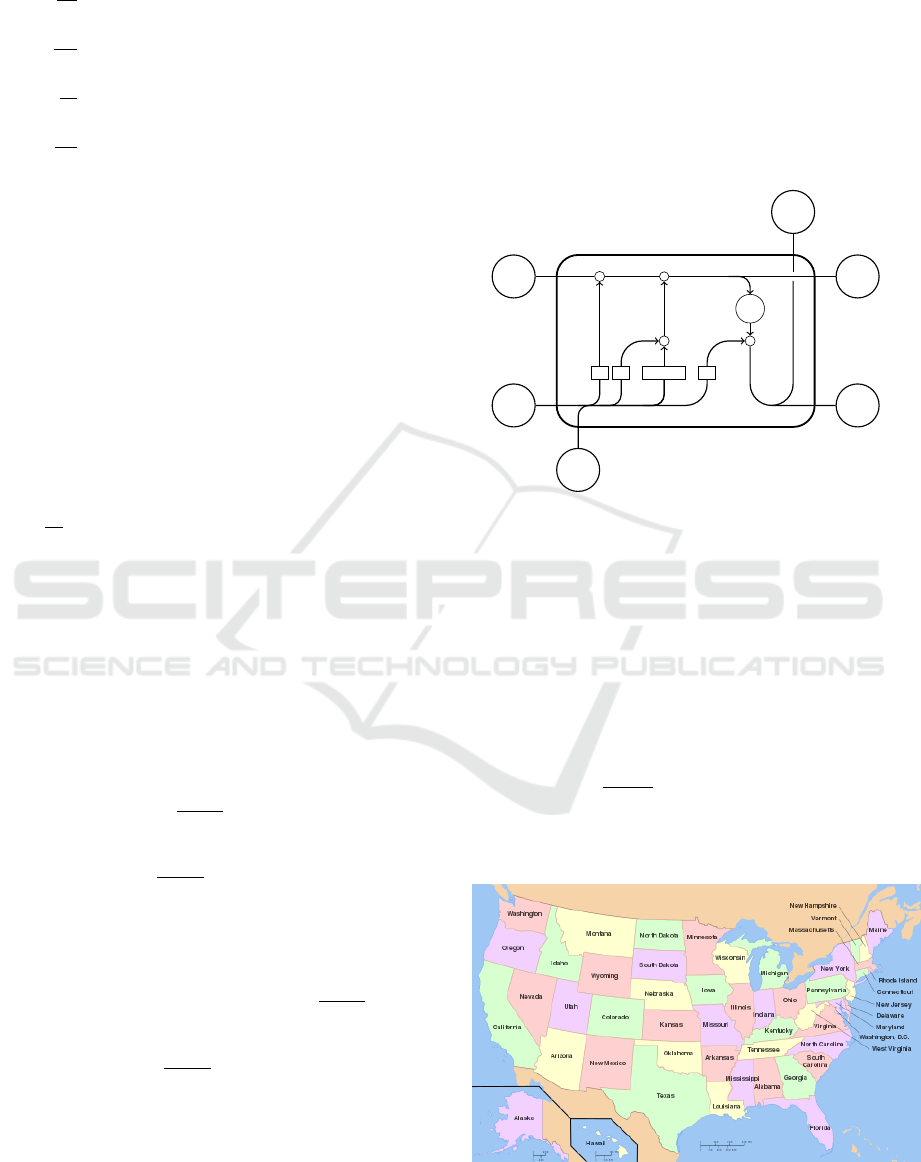
equation. To represent the latent feature from time-
varying influx of infectious individuals, we make use
of LSTM, a recurrent form of neural networks, see
Fig. 1.
σ σ
Ta nh
σ
× +
× ×
Tan h
ct-1
ht-1
xt
Input
ct
ht
ht
Output
Figure 1: LSTM cell.
3.2 Generate Edge Feature with I
e
The spatial information based on US states map (An-
drew, 2005), see Fig. 2, is formulated as an adjacent
matrix G = (g
i, j
). If two states v
i
, v
j
are neighbors
to each other, then g
i, j
= 1 otherwise is zero. With
the variables of graph information, we can define the
edge feature of state v
i
at time t:
f
i,t
=
1
∑
j
g
i, j
∑
j
g
i, j
p
∑
k=1
I
j,t−k
!
where I
j,t
is the infectious population percentage in
state v
j
at time t.
Figure 2: USA state map.
A Spatial-temporal Graph based Hybrid Infectious Disease Model with Application to COVID-19
359

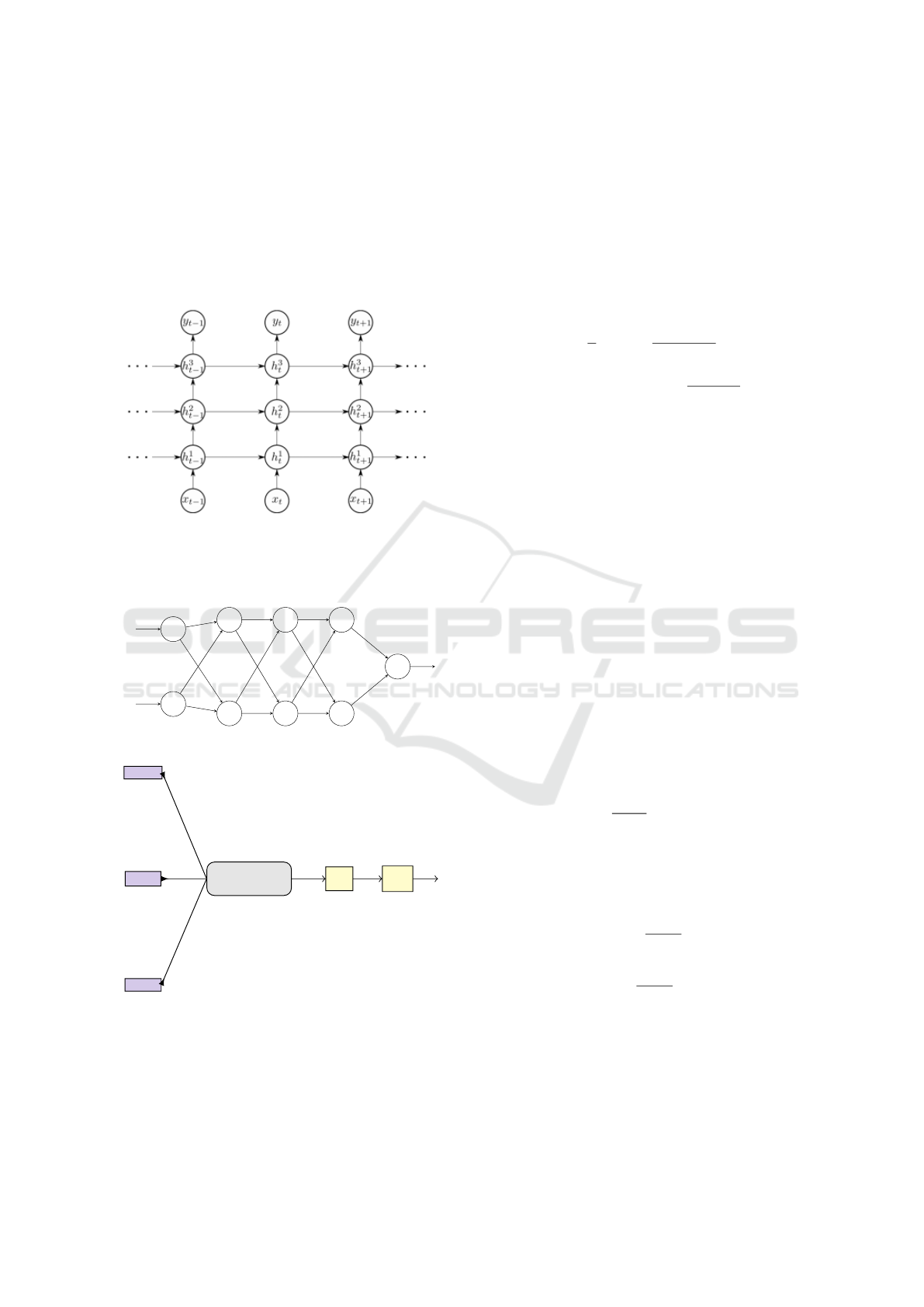
Then we design an edge-RNN composed of
stacked LSTM cells Fig. 3 with a following dense
layer Fig. 4 to output I
e
. The edge feature f
i,t
is the
input of the edge-RNN. The integrated procedure to
generate edge feature is illustrated by Fig. 5, taking
California as example. Our model, IeRNN, is named
by this design of edge-RNN for I
e
and the I-equation:
(11)I
e,t
= Dense-Layer(edge-RNN( f
i,t
))
Figure 3: Stacked LSTM cells in edge-RNN.
.
.
.
.
.
.
.
.
.
.
.
.
y
t−1
y
t−p
w
(1)
1
w
(1)
n
w
(2)
1
w
(2)
n
w
(3)
1
w
(3)
n
tanh
y
t
Input
layer
Hidden
layer
Output
layer
Figure 4: Fully connected dense layer.
Oregon
Nevada
Arizona
Edge Feature
of California
Edge
RNN
Dense
Layer
I
e
Figure 5: Generate I
e
of California.
3.3 Policy Response Modeling
During an epidemic, the rate of infection could
change as governments start responding to the epi-
demic. The infectious rate would start decreasing due
to the restrictive policy (partial or full lock-down) be-
ing put in place. We model the policy response by
changing the parameter, β
1
, in the ODE set (10). By
multiplying a control factor β
decay
(called test decay)
to β
1
, we can control the infection levels in the future
resulting from various degrees of opening policies.
The policy response β
1
is a function of time (Li
et al., 2020) to reflect no measure, restricting mass
gatherings, reopening, lock-down for different times:
(12)
β
1
(t) =
2
π
arctan

−b(t − a)
20

+ 1 + c exp

−
(t − t
0
)
2
s

where parameters a, b, c, t
0
, s are learned from fitting
historical data.
4 EXPERIMENT
We use the COVID-19 data in United States(Dong
et al., 2020) to evaluate our IeRNN model in train-
ing and testing. From (Dong et al., 2020), we find
the state level infectious data in the US. Due to the
incomplete recovered cases of US, we use the differ-
ence of cumulative cases in each state as the daily in-
fected population. Then we use the population of US
(World-Population-Review, 2020) to calculate the in-
fectious rate of each state, where we assume the popu-
lation of a state is constant during the period we con-
cerned with. The data is split into training set (133
days) and testing set (35 days) for model evaluation.
The loss function for training is mean squared er-
ror (MSE) of the output of model and true data value:
loss =
1
T + 1
T
∑
t=0
(I
t
−
ˆ
I
t
)
2
where the output of model ˆy
t
has the form (adapted
from (10)):
(13)
ˆ
I
t
= σ
1
α + (1 − σ
1
− γ)I
t−1
+ σ
2
I
e,t−1
− γ
t − t
0
P + 1
P
∑
j=0
I
t−1− j
− S
0
exp −
t − t
0
P + 1
P
∑
j=0
(β
1
I)
t−1− j
+ (β
2
I
e
)
t−1− j
!
where we have parameters (α, β
1
,β
2
,γ,σ
1
,σ
2
). Due
to the interpretations of SEIR model, these parameter
values should range in the interval [0, 1].
ICPRAM 2021 - 10th International Conference on Pattern Recognition Applications and Methods
360

We use gradient descent optimizer, Adam
(Kingma and Ba, 2015), to train our IeRNN model.
In each step, we update the weight of neural networks
model (10) and the parameters of loss function (13)
separately with different length of step and regular-
ization norms.
To assess the performance of our model, we de-
sign a series of numerical experiments to compare
the IeRNN with I-equation, temporal LSTM and
ARIMA.
Regarding model size, the IeRNN and LSTM
have about 4240 parameters while the I-equation and
ARIMA have 5 parameters.
4.1 Robustness in Parameter
Initialization
Model robustness in training is an important attribute,
so that the model performance is not sensitive to
initialization of parameters (α,β
1
,β
2
,γ,σ
1
,σ
2
) during
training. We find that the I-equation (I-model with
I
e
= 0) is not easy to learn in the sense that a sub-
optimal local minimum is often reached by gradient
descent during optimization. With coupling to RNN
(I
e
6= 0) in IeRNN, the landscape of loss function is
regularized so that a local minimum from any random
initialization gives a robust and accurate fit. Fig. 8
shows that I-equation is much less accurate in 1-day
ahead prediction than IeRNN. Fig. 9 illustrates the
same outcome in 7-day ahead prediction.
In further experiment, we train and test IeRNN
and I-equation with randomly initialized parameters
(α,β
1
,β
2
,γ,σ
1
,σ
2
). By repeating the training and test-
ing procedure for 20 times, we compare the average
MSE loss for both models. The results in Tables 1 and
2 show that IeRNN performs better for both training
loss and testing loss in 1-day ahead and 7-day ahead
predictions.
Table 1: Average MSE’s of training (testing) loss in 1-day
ahead prediction.
IeRNN I-equation
California
training 7.63e-09 8.49e-08
testing 1.26e-08 9.68e-07
Florida
training 4.24e-08 3.45e-06
testing 3.59e-08 3.97e-05
Virginia
training 3.70e-09 2.60e-08
testing 6.90e-09 1.56e-07
4.2 1-day Ahead Prediction
We compare IeRNN (with β
1
(t)), IeRNN, LSTM and
ARIMA on 1-day ahead prediction. IeRNN achieves
Table 2: Average MSE’s of training (testing) loss in 7-day
ahead prediction.
IeRNN I-equation
California
training 8.01e-09 1.32e-07
testing 9.66-09 1.62e-06
Florida
training 8.15e-09 1.49e-06
testing 9.77e-09 2.20e-05
Virginia
training 7.69e-09 8.21e-08
testing 2.03e-08 1.41e-06
lower MSE error than LSTM and ARIMA on test set.
With policy response function β
1
(t), IeRNN gives
further improvement beyond IeRNN with constant β
1
,
see Table 3.
Table 3: MSE comparison of different models on 1-day
ahead prediction.
IeRNN IeRNN LSTM ARIMA
β
1
(t)
California 1.83e-09 2.45e-09 5.00e-09 1.44e-08
Florida 6.13e-09 7.55e-09 4.68e-08 4.11e-08
Virginia 1.27e-09 1.29e-09 3.37e-09 3.74e-09
4.3 7-day Ahead Prediction
Motivated by weekly forecasting from CDC, we study
the 7-day ahead prediction task. The loss function is
modified by replacing the I-model by a 7-day delayed
version below:
ˆ
I
t
= σ
1
α + (1 − σ
1
− γ)I
t−7
+ σ
2
I
e,t−7
− γ
t − t
0
P + 1
P
∑
j=0
I
t−7− j
− S
0
exp −
t − t
0
P + 1
P
∑
j=0
(β
1
I)
t−7− j
+ (β
2
I
e
)
t−7− j
!
(14)
where the output value at time t is influenced by the
feature vector I
e
at time t − 7 and earlier. With a sim-
ilar modification of loss function, we adapt LSTM to
the 7-day ahead prediction. Table 4 compares IeRNN
and LSTM in terms of MSE on testing data.
4.4 Effect of Policy Response β
1
(t) in
Testing
To study the effect of policy response in IeRNN
model on testing data, we multiply the learned β
1
(t)
by a constant factor (called test decay) during testing.
A Spatial-temporal Graph based Hybrid Infectious Disease Model with Application to COVID-19
361

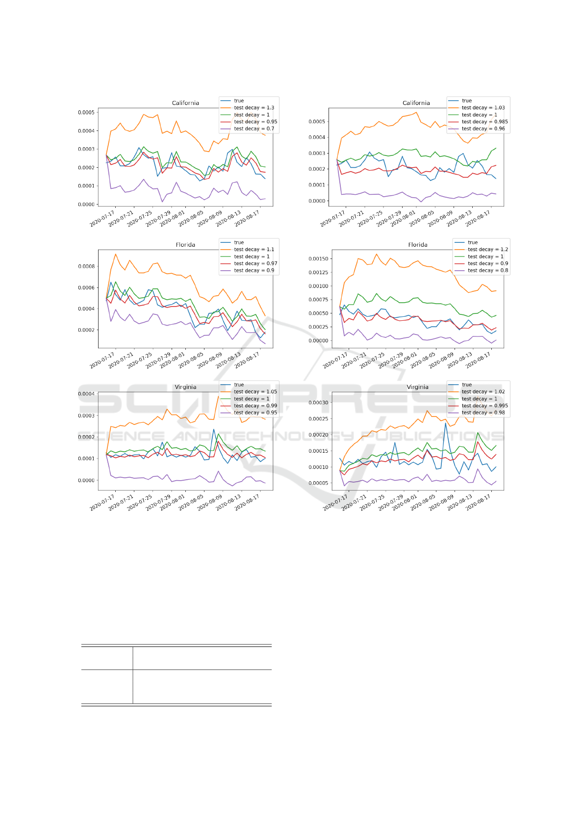
Figure 6: Effect of test decay (policy response multiplier)
in test period of 1-day ahead prediction task. The IeRNN
is trained through March 3, 2020 to July 14, 2020. The
vertical axis is fraction of newly infected people in the pop-
ulation. The horizontal axis is time in unit of days.
Fig. 6 and Fig. 7 show the impact to model predic-
tion on test data by adjusting test decay which could
control the future trend of infection.
Table 4: MSE comparison of different models on 7-day
ahead prediction.
IeRNN IeRNN LSTM
β
1
(t)
California 6.79e-09 9.84e-09 1.49e-08
Florida 4.34e-08 4.47e-08 5.74e-08
Virginia 1.16e-09 1.55e-09 1.54e-08
Figure 7: Effect of test decay (policy response multiplier)
in test period of 7-day ahead prediction task. The IeRNN
is trained through March 3, 2020 to July 14, 2020. The
vertical axis is fraction of newly infected people in the pop-
ulation. The horizontal axis is time in unit of days.
5 CONCLUSIONS
We develop a novel spatio-temporal infectious disease
model called IeRNN, which is a hybrid model con-
sisting of I-equation from SEIR driven by spatial fea-
tures. With such features and RNN dynamics as exter-
nal input to the I-equation, the robustness to parame-
ter initialization in model training is greatly improved.
In 1-day and 7-day ahead prediction, our model out-
performs standard temporal models. In future work,
ICPRAM 2021 - 10th International Conference on Pattern Recognition Applications and Methods
362

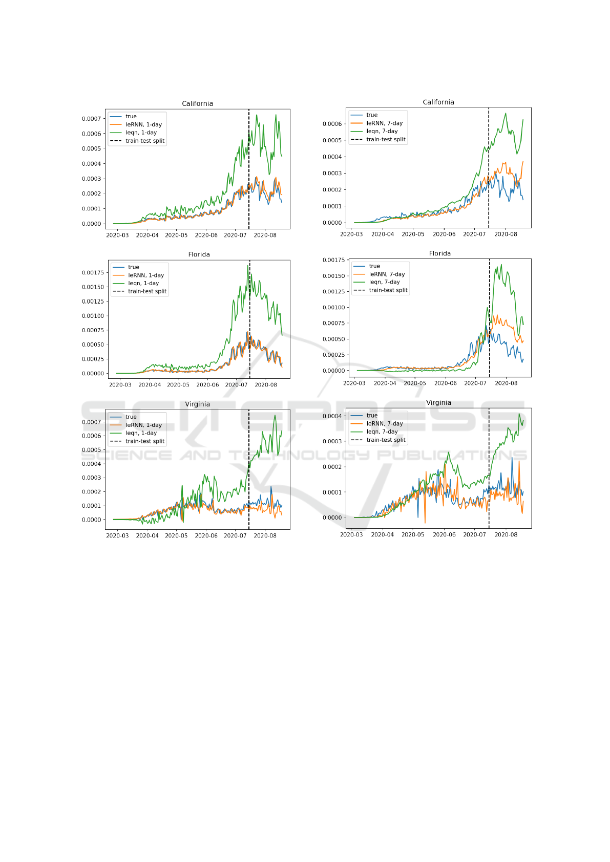
Figure 8: Comparing 1-day ahead predictions of IeRNN
and I-equation with training (testing) period to the left
(right) of the vertical dashed line. The vertical axis is frac-
tion of newly infected people in the population. The hori-
zontal axis is time in unit of days.
the social control mechanisms (Albi et al., 2020; Mor-
ris et al., 2020) could be considered to strengthen the
I-equation, as well as traffic data to expand inflow ef-
fect beyond geographic neighbors.
ACKNOWLEDGEMENTS
The work was partially supported by NSF grants IIS-
1632935, DMS-1924548.
Figure 9: Comparing 7-day ahead predictions of IeRNN
and I-equation with training (testing) period to the left
(right) of the vertical dashed line. The vertical axis is frac-
tion of newly infected people in the population. The hori-
zontal axis is time in unit of days.
REFERENCES
Albi, G., Pareschi, L., and Zanella, M. (2020). Control with
uncertain data of socially structured compartmental
epidemic models. arXiv preprint arXiv:2004.13067.
Anderson, R. and May, R. (1992). Infectious Diseases of
Humans: Dynamics and Control. Oxford University
Press, Oxford.
Andrew, C. (2005). A map of the united states, with state
names (and washington d.c.).
Deng, S., Wang, S., Rangwala, H., Wang, L., and Ning, Y.
A Spatial-temporal Graph based Hybrid Infectious Disease Model with Application to COVID-19
363

(2019). Graph message passing with cross-location
attentions for long-term ili prediction. arXiv preprint
arXiv:1912.10202.
Dong, E., Du, H., and Gardner, L. (2020). An interactive
web-based dashboard to track covid-19 in real time.
Lancet Inf Dis. 20(5):533-534. doi: 10.1016/S1473-
3099(20)30120-1.
Hethcote, H. W. (2000). The mathematics of infectious dis-
eases. SIAM Review, 42:599 – 653.
Hochreiter, S. and Schmidhuber, J. (1997). Long short-term
memory. Neural computation, 9(8):1735–1780.
Kingma, D. and Ba, J. (2015). Adam: A method for
stochastic optimization. 3rd International Conference
for Learning Representations, San Diego, 2015.
Lai, G., Chang, W., Yang, Y., and Liu, H. (2017). Model-
ing long- and short-term temporal patterns with deep
neural networks. CoRR, abs/1703.07015.
Li, M. L., Tazi Bouardi, H., Skali Lami, O., Trikalinos,
T. A., Trichakis, N. K., and Bertsimas, D. (2020).
Forecasting covid-19 and analyzing the effect of gov-
ernment interventions. medRxiv.
Li, Z., Luo, X., Wang, B., Bertozzi, A., and Xin, J. (2019).
A study on graph-structured recurrent neural networks
and sparsification with application to epidemic fore-
casting. In World Congress on Global Optimization,
pages 730–739. Springer.
Morris, D. H., Rossine, F. W., Plotkin, J. B., and Levin,
S. A. (2020). Optimal, near-optimal, and robust epi-
demic control. arXiv preprint arXiv:2004.02209.
Roosa, K., Lee, Y., Luo, R., Kirpich, A., Rothenberg, R.,
Hyman, J., Yan, P., and Chowell, G. (2020). Real-
time forecasts of the COVID-19 epidemic in China
from February 5th to February 24th, 2020. Infectious
Disease Modelling, 5:256 – 263.
Wang, B., Luo, X., Zhang, F., Yuan, B., Bertozzi, A., and
Brantingham, P. (2018). Graph-based deep model-
ing and real time forecasting of sparse spatio-temporal
data. MiLeTS ’18, London, UK, DOI: 10.475/123 4;
arXiv preprint arXiv:1804.00684.
Wang, B., Yin, P., Bertozzi, A., Brantingham, P., Osher, S.,
and Xin, J. (2019). Deep learning for real-time crime
forecasting and its ternarization. Chinese Annals of
Mathematics, Series B, 40(6):949–966.
World-Population-Review (2020). Us states population
2020.
Wu, Y., Yang, Y., Nishiura, H., and Saitoh, M. (2018). Deep
learning for epidemiological predictions. The 41st In-
ternational ACM SIGIR Conference on Research &
Development in Information Retrieval.
Yang, S., Santillana, M., and Kou, S. (2015). Accurate es-
timation of influenza epidemics using Google search
data via ARGO. Proceedings of the National Academy
of Sciences, 112(47):14473–14478.
Yu, B. and Yin, H. (2018). Spatio-temporal graph convolu-
tional networks: A deep learning framework for traffic
forecasting. Twenty-Seventh International Joint Con-
ference on Artificial Intelligence IJCAI-18.
ICPRAM 2021 - 10th International Conference on Pattern Recognition Applications and Methods
364