Real-time Monocular 6DoF Tracking of Textureless Objects using

Photometrically-enhanced Edges

Lucas Valenc¸a

1 a

, Luca Silva

1 b

, Thiago Chaves

, Arlindo Gomes

1 c

, Lucas Figueiredo

1 d

Lucio Cossio

, Sebastien Tandel

, Jo

ao Paulo Lima

3,1

, Francisco Sim

oes

4,1 e

and Veronica Teichrieb

1 f

Voxar Labs, Centro de Inform

atica, Universidade Federal de Pernambuco, Recife, Brazil

HP Inc., Porto Alegre, Brazil

Departamento de Computac¸

ao, Universidade Federal Rural de Pernambuco, Recife, Brazil

Campus Belo Jardim, Instituto Federal de Pernambuco, Belo Jardim, Brazil

Keywords:

6DoF Tracking, Edge-based, Monocular, Real-time, Model-based, Mobile, Multi-object, Augmented Reality,

Textureless, Segmentation, RGB, HSV, Single-thread.

Abstract:

We propose a novel real-time edge-based 6DoF tracking approach for 3D rigid objects requiring just a monoc-

ular RGB camera and a CAD model with material information. The technique is aimed at low-texture or

textureless, pigmented objects. It works even when under strong illumination, motion, and occlusion chal-

lenges. We show how preprocessing the model’s texture can improve tracking and apply region-based ideas

like localized segmentation to improve the edge-based pipeline. This way, our technique is able to ﬁnd model

edges even under fast motion and in front of high-gradient backgrounds. Our implementation runs on desk-

top and mobile. It only requires one CPU thread per object tracked simultaneously and requires no GPU. It

showcases a drastically reduced memory footprint when compared to the state of the art. To show how our

technique contributes to the state of the art, we perform comparisons using two publicly available benchmarks.

1 INTRODUCTION

Tracking the 6DoF pose of a 3D object through

monocular videos in real-time has been a long-time

computer vision challenge. Multiple tasks in thriving

technological ﬁelds (e.g., extended reality, robotics,

autonomous vehicles, medical imaging) require infor-

mation regarding the objects populating the environ-

ment. Real-time tracking requires high precision with

temporal consistency at every snapshot of the scene.

In addition, dynamic conditions of the real world may

impose numerous difﬁculties, such as unexpected oc-

clusions, foreground or background clutter, varying

illumination, and motion blur. Hardware challenges

are also present (e.g., lack of processing power or suf-

ﬁciently reliable scene input from available sensors).

https://orcid.org/0000-0003-2625-9857

https://orcid.org/0000-0003-2182-9208

https://orcid.org/0000-0003-3930-2754

https://orcid.org/0000-0001-9848-5883

https://orcid.org/0000-0001-9368-2298

https://orcid.org/0000-0003-4685-3634

It is also important to brieﬂy mention detection

techniques, which are often seen as complementary

to tracking works. The main difference between them

lies in the temporal consistency and computational

cost. Usually, the detection step (which can be au-

tomated or even manually aligned) provides an ini-

tial estimation for trackers to use. Unlike detectors,

trackers achieve higher efﬁciency by not needing to

search the entire frame every time, as the object is ex-

pected to be in the vicinity of where it was in the last

frame. Additionally, trackers try to make the current

frame’s estimation coherent with respect to the previ-

ous frames, generating smoother results.

Objects being tracked can vary in appearance, be-

ing considered textured if there is a signiﬁcant amount

of visual information such as internal gradients and

color variation. The lack of such information in tex-

tureless objects conﬁgures a relevant category con-

sidering how widely common these objects are (e.g.,

3D prints, industrial parts), and how suitable their

textureless surfaces are for applications such as aug-

mented reality.

Valença, L., Silva, L., Chaves, T., Gomes, A., Figueiredo, L., Cossio, L., Tandel, S., Lima, J., Simões, F. and Teichrieb, V.

Real-time Monocular 6DoF Tracking of Textureless Objects using Photometrically-enhanced Edges.

DOI: 10.5220/0010348707630773

In Proceedings of the 16th International Joint Conference on Computer Vision, Imaging and Computer Graphics Theory and Applications (VISIGRAPP 2021) - Volume 5: VISAPP, pages

763-773

ISBN: 978-989-758-488-6

763

This paper presents a novel 6DoF object tracking

technique (see Fig. 1) based on edges and photomet-

ric properties. Our technique is mainly aimed at rigid,

textureless or low-texture objects with pigmentation

(see Section 3.4). It uses previously known mate-

rial information from the input 3D model to generate

photometrically-robust local color data. This data un-

dergoes statistical simpliﬁcation in order to generalize

it, enabling matching to real-world objects. During

tracking, the color matching process then generates a

binary segmentation mask in real time. We demon-

strate that our approach is capable of matching ob-

ject edges even under motion blur or in front of high-

gradient backgrounds, helping to overcome what is

arguably the largest pitfall of edge-based tracking. We

also introduce a novel, more computationally efﬁcient

way to match object’s 2D and 3D silhouette points

and a new search range concept (Valenc¸a, 2020).

In terms of hardware, the only required input sen-

sor is a monocular RGB camera, such as a usual mid-

range commodity webcam, and a single CPU core per

object. The proposed technique is also, to the best of

our knowledge, the ﬁrst monocular real-time 6DoF

object tracker among state-of-the-art contenders to

have been shown to work in mobile devices. For this

reason, we argue that the proposed work is more suit-

able for lightweight application scenarios than cur-

rently existing methods. Additionally, most ﬁelds that

make use of object tracking commonly utilize it as

part of a larger pipeline (running simultaneously with

other algorithms). Thus, sparing resources by just us-

ing one core of the (usually multi-core) modern CPU

can be considered a desirable feat.

Our work’s main contributions are summarized as:

• A novel multi-platform edge-based approach

aimed at textureless, pigmented objects which

provides comparable precision to the state of the

art with less hardware requirements, lower run-

time, and a memory footprint orders of magnitude

smaller. The technique excels in handling illumi-

nation changes and fast motion. It also contains a

new way for edge-based tracking to isolate object

edges under blur and high-gradient backgrounds.

• Sequences using 3D printed textureless objects.

2 RELATED WORK

Due to the various tracking challenges that objects

and scenes can present, very distinct methods exist in

the literature. Feature and SLAM-based approaches,

which use feature descriptors to extract object and

scene characteristics, have been adapted to 6DoF de-

tection and tracking. These are particularly popular in

industry applications for mobile devices

, generally

coupled with 3D reconstruction (not model-based). In

the academia, ORB-SLAM2 (Mur-Artal and Tard

os,

2017) has been adapted to track 3D rigid objects (Wu

et al., 2017) in a benchmark scenario. These methods

tend to struggle with textureless objects and perform

best in unchanging scenes with ﬁxed illumination and

object position (relative to the scene).

Recently, monocular region-based approaches

have been proposed (Tjaden et al., 2018; Zhong and

Zhang, 2019; Stoiber et al., 2020), and most famously

PWP3D (Prisacariu and Reid, 2012). These tech-

niques track a whole portion of the input frame and

statistically differentiate between object and back-

ground colors to isolate a silhouette and estimate the

motion. One such method, RBOT (Tjaden et al.,

2018), can be seen as an evolution of PWP3D and is,

to our knowledge, the approach that has so far been

proven to yield the most reliable results in multiple

versatile conditions. It is suitable to a wide range of

objects and textures, and has been thoroughly evalu-

ated in multiple benchmarks. Very recently, The main

problem with real-time region-based approaches lies

in their computational cost (e.g., PWP3D relies heav-

ily on GPGPU, and RBOT on multi-threading and

GPU rendering). This parallelism bottleneck comes

to light especially for multi-object tracking. Very re-

cently, a work has proposed a sparse region-based ap-

proach that might help overcome this performance is-

sue (Stoiber et al., 2020).

Edge-based approaches have been around the

longest and tend to be more lightweight (Seo et al.,

2013). They attempt to match the model’s edges

to gradients found in the frame. The main edge-

based pipeline was popularized by RAPID (Harris

and Stennett, 1990) and a wide array of trackers (Han

and Zhao, 2019) have been developed on top of

the RAPID pipeline, including the proposed method.

Initially, RAPID-based works relied only on differ-

ences of grayscale intensity. Then, techniques like

GOS (Wang et al., 2015) started applying color anal-

ysis to regions neighboring the edges. Edge-based

techniques tend to struggle with highly textured back-

grounds, as the many gradients can cause erroneous

matching. Additionally, they are prone to fail in

cases of heavy motion where edges become blurred.

Thus, since the appearance of recent region-based ap-

proaches like RBOT, to our knowledge, edge-based

works have fallen out of the state of the art (with one

exception, which is not real-time capable) (Bugaev

et al., 2018).

For completeness sake, we shall also mention a

relevant RGB-D deep learning approach (Garon and

Apple ARKit

VISAPP 2021 - 16th International Conference on Computer Vision Theory and Applications

764

Figure 1: Our work in different scenes. Left to right: ﬂashing lights, occlusion, clipping, motion blur, multi-object, and AR.

Lalonde, 2017). It has not achieved the same runtime

speed of machine learning RGB-D trackers (Tan et al.,

2017). Still, it was shown to be reliable in scenarios

with strong occlusions or imprecise initialization. As

downsides, we must mention the hardware require-

ments (RGB-D cameras and high-end GPUs).

3 METHOD

Our method uses the object’s 3D model together with

its material information. Models are deﬁned as stan-

dard triangular meshes composed by a set of vertices,

edges, and faces, without repetition of shared edges

between faces. Materials can be assigned to the en-

tire object or to a subset of faces. Diffuse texture

images are assumed to be in RGB format with 8-

bit quantization per intensity channel. The color of

faces with no diffuse texture speciﬁed in its mate-

rial (as is the case with textureless objects such as

solid-color 3D prints) is referred to as the RGB vec-

tor C ∈ R

→ {0,··· , 255}

. Such color is speciﬁed

by the diffuse color coefﬁcient of the face’s material.

All frames are remapped to remove radial and tan-

gential lens distortion. We also assume the camera to

be precalibrated, with the focal length and principal

point expressed in pixels as the 3 × 3 intrinsic param-

eter matrix K, as per the pinhole camera model.

The extrinsic parameter matrix E describes the

6DoF transform from world to camera space and is

represented as a 3 × 4 matrix [R t]. The projection

p ∈ R

of an object point P ∈ R

can be described as

p = β(K ·(E ·

P)), with

P being its homogeneous coor-

dinate form. Additionally, β represents the conversion

between P

→ R

so that β(P) = [X /Z,Y /Z]

∈ R

The pose E

for the i

frame can be estimated

by approximating the object’s inﬁnitesimal rigid body

motion between frames. This is done by using the i

frame and the last known pose expressed by E

(i−1)

estimate ∆t = t

−t

(i−1)

and ∆R, ﬁnally obtaining E

3.1 Model Preprocessing

Before tracking begins, the 3D model is preprocessed

and has its texture simpliﬁed. This is a one-time pro-

cedure. Every model face’s diffuse texture image re-

gion (i.e., the diffuse image associated to the set of

vertices, masked by the UV coordinates associated

with each face vertex) is simpliﬁed by being quan-

tized into a 32-bin RGB probability histogram. Each

color’s probability value corresponds to the percent-

age of pixels of said color in the face’s histogram.

Colors are then ranked according to said probabil-

ity, highest ﬁrst, and stored in HSV format. They are

stored until either reaching a k

= 95% accumulated

probability limit (i.e., all stored colors for that face

represent over k

% of the face’s surface) or reaching

the k

= 3 color per face limit. For faces without dif-

fuse texture, C = 100% probability. The k

limit was

set to avoid storing unrepresentative colors and k

was set due to our textureless scope, as an upper limit

for the amount of colors and gradients per triangle.

Each face color is then assigned to every edge

within the face. Thus, every edge has a list of all col-

ors from all faces that contain it, without repetition.

The list of edges, vertices that form them, and HSV

colors they contain are then stored. The original ob-

ject model and materials are no longer utilized.

3.2 Efﬁcient Silhouette Encoding

The ﬁrst step executed in real-time for every frame

consists of encoding the 2D-3D correspondences for

the current pose. All the model’s 3D vertices are pro-

jected using the last known pose. Based on line pro-

jection properties, the 2D edges are drawn using the

projected vertices and Bresenham’s line-drawing al-

gorithm. The canvas used consists of a single-channel

32-bit image. Each pixel of a projected edge has

its intensity value corresponding to its own 3D edge

index from the edge set ξ contained in the prepro-

cessed model. This is similar to the Edge-ID algo-

rithm (Lima et al., 2009), but uses a single 32-bit

channel directly for the ID instead of splitting it in

three 8-bit channels. The resulting image is referred

as the codex. It is important to mention that our imple-

mentation does not utilize depth testing (for details,

see the Appendix).

Next, a topological border following algo-

rithm (Suzuki and Abe, 1985) is used on the codex

to extract the external-most 2D contour ζ. The con-

tour is continuous and returned in counter-clockwise

Real-time Monocular 6DoF Tracking of Textureless Objects using Photometrically-enhanced Edges

765

order. This set of pixels corresponds to the object’s

2D silhouette at the last known 6DoF pose.

Finally, the set of 2D normal vectors ϒ is deter-

mined so that ϒ

Θ(ζ

(i+1)

− ζ

(i−1)

), as ζ is circular

and continuous. The vector

Θ corresponds to the nor-

malized output of the function Θ(v) = [−y,x]

, which

returns a 2D vector orthogonal to v = [x,y]

∈ R

The normal vector is always rotated 90

clockwise.

Given the counter-clockwise property of the contour’s

continuity, this means the 2D normals will automati-

cally always point outwards from the silhouette.

To extract a 3D point P from the codex’s 2D point

p, because we only projected the edge vertices, we

need to linearly interpolate those two endpoint Z val-

ues to obtain P

. Then, P = [(p

− c

)/(P

· f ),(p

−

)/(P

· f ), P

]

(Lima, 2014), where c

, c

, and f

come from the intrinsic camera matrix K deﬁned pre-

viously. To ﬁnd those two endpoint Z values we see

the edge ID in the codex and verify in the edge array

which pair of 3D vertices compose that edge. This

operation is only performed when a match is found

for that silhouette pixel, which is more efﬁcient than

calculating all Z values using a z-buffer.

3.3 Adaptive Circular Search

In order to segment the frame, we need to estab-

lish a search range. Instead of conducting 1D linear

searches directly (as is traditional in edge-based ap-

proaches), our search is performed locally in dense

circular areas with radius r, centered around contour

points from ζ (drawing inspiration from RBOT). The

goal in our case, though, is to match the colors found

in the frame with the ones expected from that region

of the preprocessed 3D model. Additionally, instead

of sampling 3D points at random, we’re taking con-

secutive points directly from ζ in 2D. This is done to

maintain uniform contour coverage as the projected

silhouette’s length varies with z-axis translation.

Ideally, every point in ζ should be evaluated in its

own circle, covering a dense strip around the object’s

curvature. Because that is too computationally expen-

sive, we are instead sampling every r

consecutive

contour point so that every circle is always equally

re-visited by each of its neighbors, increasing cover-

age. Neighbors checking the circle area can be useful

when there’s larger motion between frames or colors

are blended due to blur.

Instead of using a ﬁxed radius value (as is com-

monly done in tracking approaches), we suggest to

change the radius according to the object’s current sil-

houette area in relation to the frame resolution. This

way, r is updated at every new pose, proportionally

to how many pixels are being occupied by the ob-

ject’s projection. This region consists of all pixels

inside (and including) ζ, referred to as A(ζ). Thus,

the amount of pixels inside this region is represented

by |A(ζ)|. The radius r can be calculated as a linear

function with limiting thresholds:

r(ζ) = min



· λ

−1

· |A(ζ)| + r



· λ





, (1)

where r

= 7 pixels is the minimum tolerable level of

detail where shapes are still discernible for our PnP-

based approach, determined empirically. The angu-

lar coefﬁcient k

= 0.002 determines how fast the ra-

dius grows with proportion to the object size. The

value of the maximum allowed radius is deﬁned as

· |A(F)|/π, where |A(F)| is the total area

(in pixels) of the input frame F and k

= 0.01, or 1%,

corresponds to the percentage of the frame that the

maximum radius is allowed to occupy. The suggested

values for k

and k

were found via experimentation

with multiple handheld objects.

Variable λ

= |A(F)|/(R

· R

) represents the

scale factor between the current resolution and R,

the base resolution (in our case VGA). It makes it

so our technique behaves uniformly under resolution

changes. Subscripts h and w represent height and

width, respectively.

Finally, λ

= min(F

)/min(R

) represents

the shortest side scale. It minimizes changes when

under different (e.g., wider or narrower) aspect ratios.

An alternative to using λ

to handle changes in aspect

ratio is to use directly-proportional elliptical search

circles, but that would divert from the circular search

concept by creating directional search bias.

3.4 Binary Segmentation

We construct a segmentation mask by evaluating ev-

ery pixel within the search circles described previ-

ously. In an ideal world, where the model texture cor-

responds exactly to what we will ﬁnd in the frame, the

binary segmentation is very straightforward. Yet, due

to the reality gap, we must establish tolerances for a

pixel’s color to be considered a match. These toler-

ances are controlled by what we call the uncertainty

coefﬁcient, or σ. The idea is that in a scenario where

we’re very sure the texture is accurate, such as in 3D

printed objects or synthetically-rendered scenes and

applications, the uncertainty (and therefore tolerance

to variation) is low. But in a real world scenario, that

tends to be larger (see Section 6.1).

The core idea of the proposed segmentation ap-

proach consists of utilizing the photometric proper-

ties of the HSV space to help in overcoming reality

gap challenges and ﬁlter pixels. By utilizing hue and

saturation information, we can more easily identify a

VISAPP 2021 - 16th International Conference on Computer Vision Theory and Applications

766

preprocessed color in cases where, if using a space

like RGB, it might not be so clear. Because we rely

on HSV, our approach focuses on pigmented objects.

Grayscale (non-pigmented) objects do not possess re-

liable hue information (see the Appendix).

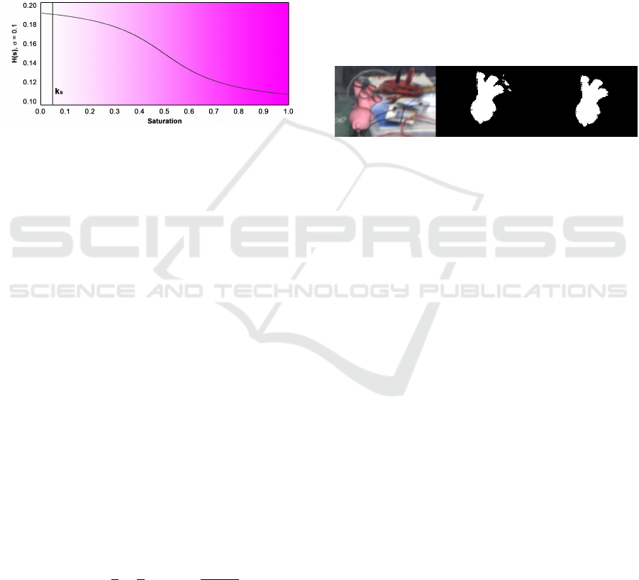
To take advantage of the HSV properties, we bor-

row a concept from region-based techniques: the

smoothed unit step function (see Fig. 2). In our case,

we want to statistically highlight the difference be-

tween regions of HSV space itself, as to continuously

regulate the uncertainty tolerance levels proportion-

ally to the amount of pigmentation present.

Figure 2: Behavior of H(s) for σ = 0.1 as saturation

changes. Desaturation threshold k

is also highlighted.

This way, a segmented frame pixel p must satisfy

the following conditions with respect to the prepro-

cessed color c in order to be set as 1, or true, in the

binary segmentation:

H(p

) ≥ d

−c

) ∧ p

> k

∧ η ≥ |p

−c

|, (2)

where subscript h and s represent the hue and satu-

ration channels, respectively. Function d

represents

the shortest distance between hue values (considering

they are cyclic) and constant k

= 0.05 represents the

minimum saturation threshold, indicating the point

where there is so little pigmentation hue is no longer

reliable (see supplementary material). The saturation

tolerance range is mapped by the logarithmic function

η = k

· ln(σ) + k

, where the vertical shift k

= 0.5

sets the log curve’s plateau at the maximum saturation

tolerance window possible, and the elasticity coefﬁ-

cient k

= 0.08 both determines how fast that plateau

will be reached and sets the function within the 0 to 1

quantization. Finally, H represents the hue tolerance

proportional to the amount of pigmentation present,

represented by a smoothed unit step function (Wang

and Qian, 2018), adapted as follows:

H(s) = σ ·



−

·tan

−1



s − 0.5



, (3)

where k

= 0.2 represents the sharpness coefﬁ-

cient (Wang and Qian, 2018).

3.5 Mask Simpliﬁcation

After every pixel in the search circles is subjected

to the binary segmentation described in the previ-

ous section, we perform an additional check to avoid

noise and erroneous background bits in the resulting

mask. First, we identify all existing external-most

contours (Suzuki and Abe, 1985) and store the largest

contour in terms of area, assumed to be the main

tracked object body (or body portion). Every contour

with area less than k

= 5% of the largest contour’s is

removed (see Fig. 3). This heuristic does not work if

the erroneous portion is connected to the main body.

From this point, we will refer to the binary mask

as Φ, so that {Φ

,Φ

} ⊆ Φ refer to the foreground

(true) and background (false) pixel subsets.

Figure 3: Mask simpliﬁcation process. From left to right:

input frame, initial segmentation, ﬁnal simpliﬁed result.

3.6 Correspondence Search and Pose

Estimation

The next step consists of searching for a match for ev-

ery point in ζ. We do this using a traditional (Drum-

mond and Cipolla, 2002; Seo et al., 2013) edge-

based linear 1D search for gradients along the nor-

mal vectors from ϒ. This search uses the kernel

ψ =



1 −1



along the parametric pixel line de-

scribed as ζ

+ dtϒ

, and can be expressed as

S(i,t) = ψ ·



+dtϒ

+d(t+1)ϒ



, (4)

where d ∈ {−1,1} corresponds to the search direction

(inwards or outwards) so that d = 1 always points out-

wards from the model contour. The parametric term

t ∈ {0,r − 2} is limited to r − 2 to avoid matching

with the edges of the circular search masks, as this in-

dicates that the accepted pixel region would continue

beyond the search range and does not correspond to

a border. These cases are usually indicative of same-

color background regions. The minimum range of 0

deals with cases where the object did not move at all.

Eq. (4) is calculated for every value of t until

a result different from 0 is obtained. When and if

that happens, the 2D-3D point tuple (µ

, ζ

+ dtϒ

)

is stored in the vector χ as a possible match candi-

date. The 3D point µ

represents the unprojected 3D

equivalent of ζ

from the codex.

Instead of alternating d values while t in-

creases (Seo et al., 2013), we guide the direction of

Real-time Monocular 6DoF Tracking of Textureless Objects using Photometrically-enhanced Edges

767

d as per Table 1. Set W = A(ζ) − R(ζ), where R(ζ)

is a mask indicating the search range, where all pix-

els for every search circle for every chosen point in ζ

are set to 1. Thus, O = W (ζ) ∩ Φ

represents whether

there seems to be an occlusion in Φ

. This is due to

no pixels in W being reachable by the search circles,

but being within the contour, so that they can only be

set if the contour was not interrupted by occlusion and

could thus be ﬁlled, as per Fig. 4.

Figure 4: Segmentation without (A) and with (B) occlusion.

If the previous pose contour point ζ

∈ Φ

, then

the search continues outwards (d = 1) otherwise, if ζ

is outside Φ

, the search goes inwards (d = −1). If

is not ﬁlled and ζ

is not in it, then it can be ei-

ther outside or inside the current pose. Thus, we ﬁrst

assume it is inside the model and, to avoid matching

the search strip, the ﬁrst match going outwards is ig-

nored, so that only the second one is valid. If no two

matches are found, then the point is likely outside the

model and we must search for the ﬁrst match inwards.

Table 1: Guidelines for directional search and matching.

∈ Φ

O = ∅ d match stored in χ

T 6 1 1

F F −1 1

F T 1 then −1 2

then 1

We would like to argue that this segmentation step

is an interesting addition to be considered for edge-

based approaches because it circumvents the back-

ground gradients problem by postponing the gradient

matching step to the binary mask. The downside re-

mains erroneous color-based segmentation, which can

be adjusted according to the limitations of the chosen

segmentation module for each technique.

Given a set of 2D-3D correspondences χ, the cur-

rent pose is estimated as the solution of a PnP problem

using a Levenberg-Marquardt optimization scheme

with the last known pose as initial estimation.

4 IMPLEMENTATION DETAILS

This section provides details of our C++ implemen-

tation. All major steps are performed using a single

CPU thread. The implementation relies on OpenCV,

which is optimized for computational efﬁciency and

multi-platform portability. Our mobile port utilizes

the same C++ code via Android’s NDK.

Every new input frame is converted to HSV and

iterated by each tracker instance 12 times. Every iter-

ation performs steps from Sections 3.2 through 3.6.

4.1 Tracking Multiple Objects

The technique has been extended to track multiple si-

multaneous objects, without compromising the frame

rate, by having each tracker instance (one object per

instance) running on a separate CPU thread. The

amount of objects that can be tracked in parallel de-

pends on the number of physical CPU cores.

Threads are managed in a producer-consumer

scheme with the same number of threads and tracker-

object instances, no instance being tied to any speciﬁc

thread. One tracking job is queued per instance at ev-

ery new frame, but are only processed after all jobs

on the previous frame have ﬁnished, making it so the

multi-object tracking is as fast as the slowest tracker

instance. The approach is not very suitable to mobile

CPUs, as cores do not usually share the same clock

speed. Thus, our Android port does not currently sup-

port multi-object tracking.

5 3DPO Sequences

We made available our real-world qualitative se-

quences which we have named the 3DPO dataset (3D

Printed Object dataset) together with CAD models

and camera calibrations

. The set has scenes with

multiple high-quality 3D-printed objects for the chal-

lenges of clutter, extreme motion, heavy occlusion,

handling, and independent object-camera motion.

6 EVALUATION

Experiments were executed in a laptop with a dual-

core Intel Core i7 7567U CPU @ 3.50 GHz, 16 GB

of RAM, and integrated Iris 650 graphics. Results are

compared to the current state of the art using the pub-

licly available implementation of RBOT

(see the Ap-

pendix for details). We have used a reality-gap uncer-

tainty σ = 0.1 on OPT and σ = 0.01 on RBOT dataset,

unless where explicitly speciﬁed.

github.com/voxarlabs/3DPO-Dataset

github.com/henningtjaden/RBOT

VISAPP 2021 - 16th International Conference on Computer Vision Theory and Applications

768

6.1 Benchmark Comparison

For benchmark comparisons we used the publicly

available datasets OPT

at 1920×1080 resolution and

RBOT dataset

in its original resolution (640 × 512).

Experiments were conducted using the area under

curve (AUC) measure as described by OPT(Wu et al.,

2017). Results can be seen in Table 2 and Fig.5.

Table 2: AUC score table for the OPT dataset.

Method Soda Chest House Ironman Bike Jet Average

Proposed 4.11 11.76 13.45 15.70 0.04 0.94 7.67

RBOT 6.62 9.41 6.84 7.36 6.44 8.74 7.57

AUC results from Table 2 show that Chest, House,

and Ironman were reliably tracked, as they contain the

least non-pigmented parts and are less textured (bet-

ter ﬁtting our scope). One interesting aspect of our

edge-based binary approach is that it is able to more

ﬁnely match the object’s silhouette than probabilistic

approaches like region-based (see Fig.5).

Figure 5: AUC curves for Chest, House, and Ironman.

Our method particularly struggled with objects

Soda, Bike, and Jet. That was expected, as these

objects are highly textured. In addition, Bike and

Jet contain many non-pigmented portions and Soda

has a highly symmetrical silhouette. In the case of

Bike (Bugaev et al., 2018) and Jet, models and tex-

tures were also not very accurate. Thus, it is safe

to say that these three objects presented a worse-case

scenario for our work (see Fig.6).

Figure 6: Failure case which shows the proposed work at-

taching itself to the pigmented portions the Bike object.

Table 3 shows more detailed results per OPT chal-

lenge. There it can be seen that the proposed work

particularly excels in handling illumination changes.

This is mostly due to our segmentation utilizing hue

information. In terms of handling motion, our tech-

nique’s ability to swiftly recover from partial loss has

been beneﬁcial (see Section 6.2).

media.ee.ntu.edu.tw/research/OPT/

cvmr.info/research/RBOT/

Table 3: AUC scores per challenge.

Object Method

Illum. Free Scale Trans- Rota-

Changes Motion Changes lation tion

Chest

Proposed 8.75 9.77 13.69 10.19 12.23

RBOT 6.64 2.43 7.08 10.86 11.67

House

Proposed 15.19 13.70 7.78 16.12 14.67

RBOT 11.36 2.05 3.40 11.02 7.82

Ironman

Proposed 16.34 10.86 14.75 14.92 16.85

RBOT 6.52 5.45 5.78 5.41 8.81

Average

Proposed 13.43 11.44 12.06 13.74 14.58

RBOT 8.17 3.31 5.42 9.10 9.94

To evaluate how the segmentation manages mo-

tion blur, we have performed a comparison between

segmented pixels and ground truth masks using all

Level 5 motion (fastest) OPT sequences. Results in

Table 4 show that our approach successfully handles

blur, overcoming the blurred-edges problem of edge-

based techniques by using the pigmented information.

Table 4: Average results for motion blur segmentation test.

Measure Chest House Ironman

False Negatives (%) 3.50 1.98 6.82

True Positives (%) 98.75 96.99 96.74

We also performed combined tests to understand

the impact of dynamic radii. The test compared vari-

ations on search range (ﬁxed) to Eq.(1) in the Scale

Changes (zoom) scenes of the OPT dataset and the

Cat scene from the RBOT dataset. Table 5 shows dy-

namic radius is preferable for generality purposes.

Table 5: Results for different search ranges (in px).

Object

AUC or RBOT Score

r = r

/4 r = r

/2 r = r

Eq.(1)

Chest 13.65 13.71 13.90 13.90 13.69

House 2.48 7.72 7.81 8.15 7.78

Ironman 14.03 15.63 11.59 5.92 14.75

Average 10.05 12.35 11.10 9.32 12.07

Cat 57.90 67.30 94.10 88.70 97.20

Next, we use the textureless pigmented objects

from RBOT’s proposed dataset together with its pro-

posed metric (Tjaden et al., 2018) on the scene reg-

ular to evaluate robustness to similar-color back-

grounds by varying σ tolerance (see Table 6).

Numbers for the object Cat show that the pro-

posed work excels in handling similar-color back-

ground when there’s little uncertainty, even surpass-

ing RBOT’s high score, but suffers from background

matching otherwise. Such low uncertainty values are

only possible because the materials are very accurate

to the objects, which means our technique requires

high-quality 3D model materials to perform well un-

Real-time Monocular 6DoF Tracking of Textureless Objects using Photometrically-enhanced Edges

769

Table 6: Evaluation on varying σ values. Percentages S, TP,

and FN stand respectively for score (Tjaden et al., 2018),

and averages of true positives and false negatives (in %)

for the segmented pixels with respect to the ground truth

segmentation masks.

Object

Proposed (varying σ values)

RBOT

0.10 0.05 0.01

S TP FN S TP FN S TP FN S

Ape 36.7 82.6 9.5 48.4 92.5 7.6 47.4 98.1 33.5 85.2

Duck 43.8 96.2 5.5 52.2 99.7 6.1 44.9 100.0 21.6 87.1

Cat 13.5 43.7 18.8 50.4 81.2 2.7 97.2 99.5 7.1 95.5

Squirrel 25.4 67.8 18.5 37.5 77.2 15.5 70.5 97.8 34.2 99.2

der similar-color backgrounds. Ape and Duck were

precisely segmented as well, but their quick-rotating,

simple silhouettes created inconsistencies in the es-

timated poses. Squirrel was not properly segmented

even at low uncertainty due to large portions of same-

color background, which is a limitation of our seg-

mentation approach (different from similar-color).

We also evaluated the different challenges of the

RBOT dataset for the Cat object, still using RBOT’s

metric. Results from Table 7 show our technique han-

dles the challenges comparably to RBOT.

Table 7: Comparison of RBOT scores per challenge for the

Cat object (higher is better).

Method Regular Dynamic Light Occlusion Average

Proposed 97.2 97.0 87.0 93.7

RBOT 95.5 95.2 90.1 93.6

One thing to note is that RBOT’s metric is very

strict, resetting the tracker when it is not necessar-

ily lost. Thus, to show how the proposed technique

is able to recover from partial tracking losses on its

own, we have used a no-reset methodology (Garon

and Lalonde, 2017) on the RBOT dataset, and plotted

the translation and rotation errors separately for the

regular and occlusion scenes, without ever resetting

the trackers since the ﬁrst frame. Results from Fig. 7

show that our work is always able to recover the ob-

ject’s position (translation), whereas RBOT is unable

to recover since the ﬁrst loss.

Figure 7: Recovery from partial loss results.

Because detection module calls are usually com-

putationally expensive, this reduced need is highly

desirable. In addition, this adds ﬂexibility to mi-

nor losses right from the start or the tracking pro-

cess, meaning there’s less requirement for a robust

detection module. This ﬁts well with our proposed

low hardware requirement application scenario, espe-

cially considering that popular mobile trackers can be

manually-aligned by a user

and that state-of-the-art

detectors use deep learning and powerful GPUs.

6.2 Imprecise Initialization

To further understand how robust our technique is

to an imprecise previous pose, we have conducted

the very extensive Imprecise Initialization test (Garon

and Lalonde, 2017). For this test, 10 frames were

selected at random from the sequence Slow of the

3DPO dataset, which has 1155 frames at 30 Hz. This

sequence (unlike OPT ones) has a lot of clutter and

background gradients. Unlike the RBOT dataset’s,

the sequence is also not synthetic, containing motion

blur (an important aspect for temporally-consistent

real-time tracking). It consists of smooth camera

movements around a still Green Bunny, with compre-

hensive camera rotations and translations while mov-

ing closer and farther away from the object. Ground

truth was obtained with the help of ArUco markers.

Initial pose rotation and translation perturbations

are measured separately. Rotation perturbations range

from 5 to 60

and are incremented 5

at a time. Trans-

lation perturbations range from 10 to 130 mm in 10

mm increments. For each increment, 40 random sam-

ples are taken. Before computing the error, the tracker

is called 15 times for each frame to take the temporal

factor into consideration. Mean and standard devia-

tion for the L2 norms of the errors (with respect to the

ground truth) of each of the 10 sample for each of the

perturbations are plotted in Fig. 8.

The proposed technique has achieved consistent

translation robustness for up to 60 mm, which corre-

sponds to roughly 30% of the model’s size. For ro-

tation, the technique achieved constantly reliable re-

sults for up to 15

perturbation. The deep learning

work that ﬁrst proposed this methodology has also

performed well in this test (Garon and Lalonde, 2017)

(albeit using a different RGB-D sequence and object).

It achieved robustness levels of 100 mm and 30

. In

their case, though, all perturbation averages (even the

smallest ones) had at least 8 mm and 8

of error. This

is a good illustration of the trade-offs between geo-

metric and machine learning methods. The similar-

ity between these very different approaches is that

Vuforia Model Targets

VISAPP 2021 - 16th International Conference on Computer Vision Theory and Applications

770

Figure 8: Initial perturbation test. Lines represent the aver-

age error. Margins represent the standard deviation.

both are supplied with some sort of previous knowl-

edge regarding the model’s color and texture. Model-

based techniques do not tend to directly assess this is-

sue, simply falling back to a costly detection module.

Since real-world applications usually can not count

with a ground truth value, robustness to detection er-

ror is a relevant factor and should not be overlooked.

This serves as argument for using texture information

alongside geometry on model-based approaches.

6.3 Performance and Scalability

The ﬁrst frame from the RBOT dataset sequence regu-

lar and the object Cat (with 2500 vertices) were used

for this test. More object instances were added on

top of the same object to simulate a multi-object sce-

nario. The proposed work’s memory requirement was

orders of magnitude smaller than the state of the art’s,

at ∼ 10 MB per object tracked simultaneously, on

top of a baseline value ∼ 10 MB. RBOT’s memory

consumption was ∼ 4.3 GB per object, which makes

multi-object impractical for most low-end devices. In

terms of runtime, RBOT scaled linearly with ∼ 70 ms

per new object. The proposed work had an initial run-

time of ∼ 30 ms, with approximately ∼ 3 ms per new

object until a limit of 3 objects (amount of threads

able to run in parallel efﬁciently on our dual-core

CPU). Afterwards, our work’s runtime scaled linearly

with ∼ 30 ms per new object.

The second test had a similar setup but used only

one object at a time. Cat objects with different sim-

pliﬁcation levels (amount of vertices) were used, as

follows: 2500, 5000, 7500, 10000, 12500. RBOT

scaled at ∼ 4.3 GB of RAM per new 2500 vertices,

whereas the proposed work showed no signiﬁcant dif-

ference, staying at about 20 MB. In terms of runtime,

RBOT scaled ∼ 10 ms per 2500 vertices from a base-

line of ∼ 70 ms. The proposed work scaled about 2

ms per 2500 vertices, from a baseline of ∼ 30 ms.

Our single-object mobile port ran at ∼ 50 ms on a

Samsung Galaxy S10 phone.

Our work averaged roughly 2.5 ms per pipeline

iteration, consisting of: encoding, segmentation,

matching, and pose estimation. Preprocessing aver-

aged 112 ms per 100 triangles with diffuse texture and

3 ms for those without.

7 CONCLUSION

We have presented a novel edge-based 6DoF track-

ing technique focused on textureless, pigmented ob-

jects. Our work, for the intended scope of objects,

achieves comparable results to the present state of

the art while surpassing it in relevant aspects. Our

technique particularly excels in challenges like illu-

mination changes, motion, and recovering from im-

precise poses. It is also single-core, RGB-only, and

much more lightweight, thus more well suited for

less-powerful hardware. We have also proposed a

new way to avoid ﬁxed search ranges, an efﬁcient sil-

houette encoding technique, a study on using mate-

rial information for model-based 6DoF object track-

ing, and a new segmentation step which handles prob-

lems such as background gradients and gradients lost

to motion blur. Finally, we have made available se-

quences focused on 3D printed textureless objects that

we hope can enrich further research.

As future work, our technique’s main limita-

tions have proven to be symmetry, which can be

aided by photometric constraints (Zhong and Zhang,

2019); and imprecise textures along with similar or

same-color backgrounds, which can be tackled by

using temporal foreground-background segmentation

strategies as performed by region-based approaches.

ACKNOWLEDGEMENTS

This research was partially funded by Conselho Na-

cional de Desenvolvimento Cient

ıﬁco e Tecnol

ogico

(CNPq) (process 425401/2018-9) and HP Brasil

Ind

ustria e Com

ercio de Equipamentos Eletr

onicos

Ltda. with resources from the ﬁscal beneﬁt of the

Brazilian Law n

8.248, from 1991 (Brazilian Infor-

matics Law). The authors thank Voxar Labs mem-

bers Lucas Maggi, Rafael Roberto, Gutenberg Bar-

ros, Kelvin Cunha, Heitor Felix, and Thiago Souza

for helpful discussions. Tsang Ing Ren and Ricardo

Barioni are also thanked for helpful discussions as

well as for proofreading this manuscript. Finally,

Henning Tjaden, Bogdan Bugaev, and Po-Chen Wu

Real-time Monocular 6DoF Tracking of Textureless Objects using Photometrically-enhanced Edges

771

are thanked for helping the authors better understand

RBOT and OPT.

REFERENCES

Bugaev, B., Kryshchenko, A., and Belov, R. (2018). Com-

bining 3d model contour energy and keypoints for ob-

ject tracking. In Proceedings of the European Con-

ference on Computer Vision (ECCV), pages 53–69. 2,

Drummond, T. and Cipolla, R. (2002). Real-time visual

tracking of complex structures. IEEE Transactions on

pattern analysis and machine intelligence, 24(7):932–

946. 5

Garon, M. and Lalonde, J.-F. (2017). Deep 6-dof track-

ing. IEEE transactions on visualization and computer

graphics, 23(11):2410–2418. 2, 8

Han, P. and Zhao, G. (2019). A review of edge-based 3d

tracking of rigid objects. Virtual Reality & Intelligent

Hardware, 1(6):580–596. 2

Harris, C. and Stennett, C. (1990). Rapid-a video rate object

tracker. In BMVC, pages 1–6. 2

Lima, J. P., Teichrieb, V., Kelner, J., and Lindeman, R. W.

(2009). Standalone edge-based markerless tracking of

fully 3-dimensional objects for handheld augmented

reality. In Proceedings of the 16th ACM Symposium

on Virtual Reality Software and Technology, pages

139–142. 3

Lima, J. P. S. d. M. (2014). Object detection and pose es-

timation from rectiﬁcation of natural features using

consumer rgb-d sensors. 4

Mur-Artal, R. and Tard

os, J. D. (2017). Orb-slam2:

An open-source slam system for monocular, stereo,

and rgb-d cameras. IEEE Transactions on Robotics,

33(5):1255–1262. 2

Prisacariu, V. A. and Reid, I. D. (2012). Pwp3d: Real-time

segmentation and tracking of 3d objects. International

journal of computer vision, 98(3):335–354. 2

Seo, B.-K., Park, J., Park, H., and Park, J.-I. (2013). Real-

time visual tracking of less textured three-dimensional

objects on mobile platforms. Optical Engineering,

51(12):127202. 2, 5

Stoiber, M., Pfanne, M., Strobl, K. H., Triebel, R., and

Albu-Schaeffer, A. (2020). A sparse gaussian ap-

proach to region-based 6dof object tracking. In Pro-

ceedings of the Asian Conference on Computer Vision.

Suzuki and Abe (1985). Topological structural analy-

sis of digitized binary images by border following.

Computer vision, graphics, and image processing,

30(1):32–46. 3, 5

Tan, D. J., Navab, N., and Tombari, F. (2017). Look-

ing beyond the simple scenarios: Combining learn-

ers and optimizers in 3d temporal tracking. IEEE

transactions on visualization and computer graphics,

23(11):2399–2409. 3

Tjaden, H., Schwanecke, U., Sch

omer, E., and Cremers,

D. (2018). A region-based gauss-newton approach to

real-time monocular multiple object tracking. IEEE

transactions on pattern analysis and machine intelli-

gence, 41(8):1797–1812. 2, 7, 8, 11

Valenc¸a, L. (2020). Real-time 6dof tracking of rigid 3d ob-

jects using a monocular rgb camera. Bachelor’s thesis,

Universidade Federal de Pernambuco. 2

Wang, C. and Qian, X. (2018). Heaviside projection–based

aggregation in stress-constrained topology optimiza-

tion. International Journal for Numerical Methods in

Engineering, 115(7):849–871. 5

Wang, G., Wang, B., Zhong, F., Qin, X., and Chen, B.

(2015). Global optimal searching for textureless 3d

object tracking. The Visual Computer, 31(6-8):979–

988. 2

Wu, P.-C., Lee, Y.-Y., Tseng, H.-Y., Ho, H.-I., Yang, M.-H.,

and Chien, S.-Y. (2017). [poster] a benchmark dataset

for 6dof object pose tracking. In 2017 IEEE Interna-

tional Symposium on Mixed and Augmented Reality

(ISMAR-Adjunct), pages 186–191. IEEE. 2, 7

Zhong, L. and Zhang, L. (2019). A robust monocular 3d ob-

ject tracking method combining statistical and photo-

metric constraints. International Journal of Computer

Vision, 127(8):973–992. 2, 9

APPENDIX

Depth Testing

Because we’re only interested in the outermost 2D sil-

houette edges, overlap is infrequent. Objects with

rounded edges do not contain 2D silhouette edges

overlapping. Objects with straight-angled edges (such

as boxes) avoid signiﬁcant silhouette overlap due to

perspective projection. To validate this, we imple-

mented a simple CPU-based z-buffer. As expected,

for rounded-edge objects it made little to no differ-

ence, and for the straight-angled ones in scenes where

the edges were overlapping results were slightly bet-

ter. Yet, to our surprise, depth-testing made results

much worse when dealing with rotations. A possible

explanation is that by allowing some edge overlap, we

can better segment colors that are not directly visible,

but that can appear with a small rotation. Thus, as not

including depth testing made our work both faster and

more precise, we have opted to not utilize it.

Saturation Threshold

By deﬁnition, HSV space only has overlap in hue val-

ues when there is zero pigmentation present, in which

case all hue values can lead to the same color. That is

not true in the real world, though, where illumination,

materials, camera sensors, and color-conversion algo-

rithms play a role in the ﬁnal color. This concept can

VISAPP 2021 - 16th International Conference on Computer Vision Theory and Applications

772

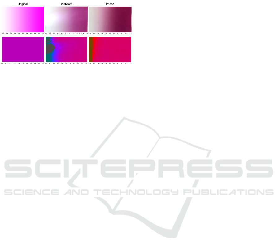
be better illustrated via a print-scan attack. Except,

instead of a scanner, we have used a webcam and a

smartphone (see Fig. 9).

Figure 9: Illustration of hue unreliability as saturation de-

creases. Top row shows the full RGB images, bottom row

the isolated hue channel.

Publicly Available Implementations

As far as we are aware (as of the time of the writing of

this paper), the best publicly available real-time RGB

6DoF trackers, which are commonly used for com-

parisons, are PWP3D, GOS, and RBOT.

PWP3D is nearly 10 years old and has since in-

spired and been surpassed by newer works, especially

RBOT, which has compared itself to it extensively.

Thus, adding PWP3D to the comparison would not

accurately represent the current state of the art.

As for GOS, it is also fairly outdated, having in-

spired newer techniques. Still, as far as we know,

no newer techniques built on top of it have a pub-

licly available implementation. In our tests, GOS’s

results averaged below 35% on the RBOT dataset

for all objects in every scene (with the reset metric).

GOS stayed below 1% without a reset. It was com-

pletely unable to recover and extremely sensitive to

motion, which caused it to fail almost immediately in

all 3DPO sequences when the objects or the camera

were moved. Thus, we felt it was out of place in the

comparison.

Next, we are going to explain why our results us-

ing the publicly available implementation of RBOT

on the OPT dataset are lower than what is reported in

RBOT’s paper (Tjaden et al., 2018). First, it is impor-

tant to note that we did manage to reproduce RBOT’s

paper’s results for the RBOT dataset. We also con-

ﬁrmed our AUC metric to be correct by reproducing

the OPT results of other works which used the pub-

licly available implementation of GOS. Upon contact-

ing the authors of RBOT, we were informed our AUC

metric seemed correct, but that OPT objects needed

some resampling to work with the publicly available

implementation of RBOT. Unfortunately, the authors

did not have access to the modiﬁed objects anymore.

In our attempts, we were unable to make the publicly

available implementation of RBOT reach the OPT

scores reported in the paper, so we decided to use

the best results we were able to get. There was no

way around this issue, as we needed to run the tech-

nique to build the AUC curves and conduct challenge-

speciﬁc tests. Still, we want to make it clear that

RBOT’s publicly available implementation does work

very robustly (even in our highly challenging 3DPO

sequences). It is also important to note that these OPT

results are still comparable to the best publicly avail-

able real-time monocular 6DoF trackers.

Real-time Monocular 6DoF Tracking of Textureless Objects using Photometrically-enhanced Edges

773