
3D Reconstruction of Deformable Objects from RGB-D Cameras: An
Omnidirectional Inward-facing Multi-camera System
Eva Curto
a
and Helder Araujo
b
Institute for Systems and Robotics, University of Coimbra, R. Silvio Lima, Coimbra, Portugal
Keywords:
Reconstruction, RGB-D, Omnidirectional, Multi-camera, Deformations.
Abstract:
This is a paper describing a system made up of several inward-facing cameras able to perform reconstruction of
deformable objects through synchronous acquisition of RGBD data. The configuration of the camera system
allows the acquisition of 3D omnidirectional images of the objects. The paper describes the structure of the
system as well as an approach for the extrinsic calibration, which allows the estimation of the coordinate
transformations between the cameras. Reconstruction results are also presented.
1 INTRODUCTION
In this paper a system for the 3D reconstruction of de-
formable objects is described. The system is made up
of several inward-facing cameras to allow for the ac-
quisition of the whole surface of the object. The sys-
tem performs the synchronous and time-stamped ac-
quisition of RGB-D images enabling the synchronous
acquisition of 3D images of deformations. Therefore,
the main contribution of this work is the assembly of
the system itself, putting together and setting up the
appropriate hardware and software.
The first algorithms for RGB-D-based dense 3D
geometry reconstruction were developed only for
static scenes. (Curless and Levoy, 1996) introduced
the fundamental work of volumetric fusion and in-
spired the most modern approaches. The ability to
provide real-time RGB-D reconstruction appears in
2002 with a system based on a 60 Hz structured-
light rangefinder (Rusinkiewicz et al., 2002). Al-
though it is no longer a recent algorithm, KinectFu-
sion (Newcombe et al., 2011) had a significant impact
on the computer graphics and vision communities.
This work was the basis for many new methods of
3D reconstruction of static and dynamic scenes. They
proposed the fusion of all data streamed from a Kinect
sensor into a single global implicit surface model of
the observed (static) scene in real-time. The current
sensor pose is simultaneously obtained by tracking
the live depth frame relative to the global model us-
a
https://orcid.org/0000-0002-0477-0091
b
https://orcid.org/0000-0002-9544-424X
ing a coarse-to-fine Iterative Closest Point (ICP) al-
gorithm, which uses all the observed depth data avail-
able. The real-time system of (Whelan et al., 2016)
is capable of capturing comprehensive dense globally
consistent surfel-based maps of room scale environ-
ments. The online BundleFusion approach of (Dai
et al., 2017) allows a robust pose estimation, optimiz-
ing per frame for a global set of camera poses by con-
sidering the complete history of RGB-D input with an
efficient hierarchical method.
The first approach to handle online deformable
tracking of arbitrary general deforming objects was
the template-based method presented by (Zollh
¨
ofer
et al., 2014). In VolumeDeform (Innmann et al.,
2016), they propose using sparse RGB feature match-
ing to improve tracking robustness and handle scenes
with a little geometric variation. Besides, they pro-
pose an alternative representation for the deforma-
tion warp field. Unlike DynamicFusion (Newcombe
et al., 2015), VolumeDeform uses the same volumet-
ric model to represent the reconstructed space. The
previous methods, (Newcombe et al., 2015), (Inn-
mann et al., 2016), achieved excellent results. How-
ever, they have a few limitations. The intermittent
conversion from Signed Distance Field (SDF) to mesh
for correspondence estimation leads to loss of accu-
racy, computational speed, and the capability to cap-
ture topological changes conveniently. Additionally,
both require 6D motion to be estimated per grid point,
while a 3D flow field is sufficient in Miroslava et al.
(Slavcheva et al., 2017) method - KillingFusion - due
to the dense smooth nature of the SDF representation
and the use of alignment constraints directly over the
544
Curto, E. and Araujo, H.
3D Reconstruction of Deformable Objects from RGB-D Cameras: An Omnidirectional Inward-facing Multi-camera System.
DOI: 10.5220/0010347305440551
In Proceedings of the 16th International Joint Conference on Computer Vision, Imaging and Computer Graphics Theory and Applications (VISIGRAPP 2021) - Volume 4: VISAPP, pages
544-551
ISBN: 978-989-758-488-6
Copyright
c
2021 by SCITEPRESS – Science and Technology Publications, Lda. All rights reserved
field. Therefore, KillingFusion provides a non-rigid
reconstruction pipeline, based on a single data repre-
sentation – SDF, which does not require explicit cor-
respondences and can handle topological changes.
The previous method employs a combination of
two regularizers, which are challenging to balance
and thus result in over-smoothing and loss of high-
frequency details. SobolevFusion (Slavcheva et al.,
2018) proposes to define the gradient flow in Sobolev
space H
−1
instead of a gradient flow based on an L
2
inner product, which is known to be susceptible to lo-
cal minima.
This section introduced the work discussed in this
paper as well as referred some state-of-art techniques
in 3D reconstruction. This paper has the follow-
ing structure: Section 2 describes the camera’s sys-
tem and the surrounding setup and explains how the
cameras were synchronized by hardware. The third
section explains the method of extrinsic calibration
used to obtain the relative position and orientation.
Then, in Section 4, we have the reconstruction phase
described and illustrated with reconstructed objects.
The final considerations of this paper are stated in sec-
tion 5.
2 SYSTEM DESCRIPTION
2.1 Cameras
Our camera system is composed of four Intel Re-
alsense D415 cameras. The choice of these cameras
took into account several factors:
• Low cost;
• The D415 come with Intel’s RealSense SDK 2.0,
which is an open-source, cross-platform SDK;
• Their field of view is well suited for high accuracy
applications such as 3D scanning;
• The rolling shutter on the depth sensor allows us
to have highest depth quality per degree.
• Theses cameras can all be hardware synchronized
to capture at identical times and frame rates.
Considering that this work proposes the omnidirec-
tional reconstruction of objects, these specifications
are satisfactory for the applications envisaged.
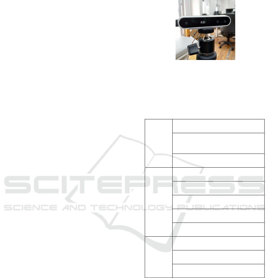
The D415, showed in Figure 1, has two main com-
ponents, the vision processor and the depth module.
The vision processor D4 is either on the host proces-
sor motherboard or on a discrete board with either
USB3.0 Gen1 or MIPI connection to the host proces-
sor. The depth module includes left and right imagers
Figure 1: Image of a RealSense D415 camera.
for stereo vision with the optional IR projector
and RGB color sensor.
The essential specifications of the D415 camera are
indicated in Table 1.
Table 1: Specifications of Intel RealSense D415.
Features
Use Environment:
Indoor/Outdoor
Image Sensor Technology:
Rolling Shutter,
1.4µm × 1.4µm pixel size
Maximum Range:
Approx. 10 meters.
Depth
Depth Technology:
Active IR Stereo
Minimum Depth Distance (Min-Z):
0.16m
Depth Field of View (FOV):
65
◦
±2
◦
× 40
◦
±1
◦
× 72
◦
±2
◦
Depth Output Resolution:
Up to 1280 × 720
Depth Frame Rate:
Up to 90 fps
RGB
RGB Sensor Resolution:
1920 × 1080
RGB Sensor FOV (H x V x D):
69.4
◦
× 42.5
◦
× 77
◦
(±3
◦
)
RGB Frame Rate:
30 fps
2.2 Experimental Setup
Each camera is mounted on a C clamp camera sup-
port, which is fixed to the table. The cameras are
equally distant between neighboring cameras since
we intend to maximize the horizontal fields of view.
The objects that will be reconstructed are illuminated
by led light in addition to natural light. In order to
avoid problems with specular reflections that could
induce more noise in RGBD acquisition and conse-
quently conduce to poor reconstruction results, we
opted to use a metallic table painted with a matte
black color. Matte allows avoiding specular reflec-
3D Reconstruction of Deformable Objects from RGB-D Cameras: An Omnidirectional Inward-facing Multi-camera System
545
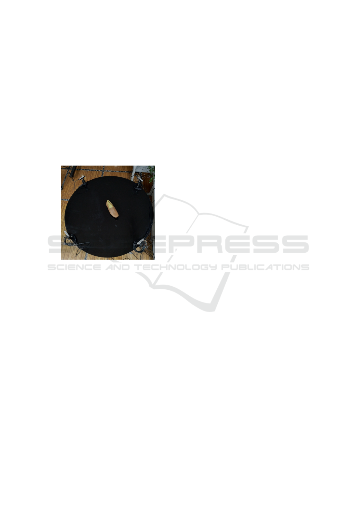
tions while metallic allows for the absorption of the
IR energy.
The synchronous acquisition of RGB-D images
from multiple cameras (four in the case) requires a
host system with enough processing power to read
from the USB ports streaming the high-bandwidth
data, and doing some amount of the real-time post-
processing, rendering, and analysis. All the work
from the data acquisition, calibration to the recon-
struction was made on a PC. This was a processor
with a Intel Core i9-9900k CPU @ 3.60GHz x 16,
a GeForce RTX 2070/PCle/SSE2, running Ubuntu
16.06 LTS.
The setup described in this section is shown in
Figure 2.
Figure 2: Picture of the omnidirectional camera system.
2.3 Hardware Synchronization
One of the requirements for our setup is the synchro-
nization between cameras, since it should also per-
form the estimation of 3D deformations.
Hardware synchronization is described in
(Grunnet-Jepsen et al., 2018), from Intel. Following
this reference, we connected the cameras via synchro-
nization cables, considering three of the cameras as
slaves and the fourth one as master. For each camera,
depth and color frames are saved as well as the
metadata. For each frame the following information
is saved: the serial number of the camera, the type
of stream (color or depth), the frame timestamp,
the sensor timestamp, the actual exposure, the gain
level, the boolean value of auto-exposure, the time of
arrival, the backend timestamp and the actual fps.
Using a hub to connect the four cameras to the
PC, the higher resolution that we achieve with the
hardware synchronization and all the color and depth
streams activated was 640 × 360. Thus, all the acqui-
sitions were made with this resolution setting.
3 EXTRINSIC CAMERA
CALIBRATION
This section begins with a brief description of the
extrinsic calibration. Then the multi-camera method
used is described.
3.1 Theory
Considering m cameras and n object points
˜
X
˜
X
˜
X
j
=
[X
j
, Y
j
, Z
j
, 1]
T
, j = 1, ..., n. We assume the pinhole-
camera model. The 3D points
˜
X
˜
X
˜
X
j
are projected to 2D
image points ˜x
˜x
˜x
i
j
as
λ
i
j
u
i
j
v
i
j
1
= λ
i
j
˜x
˜x
˜x
i
j
= P
i
˜
X
˜
X
˜
X
j
, λ
i
j
∈ R
+
(1)
where u, v are pixel coordinates, λ
i
j
the scale factors
and P
i
is the projection matrix of a given camera. This
3 x 4 matrix has 11 degrees of freedom. This projec-
tion matrix can be further decomposed as:
P
i
= K
i
[R
i
t
i
], (2)
where K
i
is the matrix of the intrinsic parameters, R
i
is the rotation matrix relative to the world coordinate
system and t
i
is the translation vector relative to the
world coordinate system.
We aim at estimating the relative positions and ori-
entations between the reference coordinate systems of
the depth cameras. The relative positions and ori-
entations are described by 6 parameters, being 3 for
rotation and 3 for translation. These are the exter-
nal/extrinsic parameters. In the case of this setup the
intrinsic parameters as well as the extrinsic parame-
ters between the cameras of each stereo pair and the
rgb camera and depth cameras are obtained from the
RealSense SDK. Then, the goal of the calibration is
to estimate the relative rotations and translations be-
tween the four different depth cameras (each of which
uses a coordinate system attached to the left camera of
each pair).
Figure 3 shows a schematic diagram of a four-
camera setup.
3.2 Overview of the Multi-camera
Method
The point clouds obtained by each depth camera are
expressed in their coordinate system. To obtain the
relative transformation we based our approach on the
method described in (Matsumoto and Aguilar-Rivera,
2018). This multi-camera calibration method is, on
VISAPP 2021 - 16th International Conference on Computer Vision Theory and Applications
546
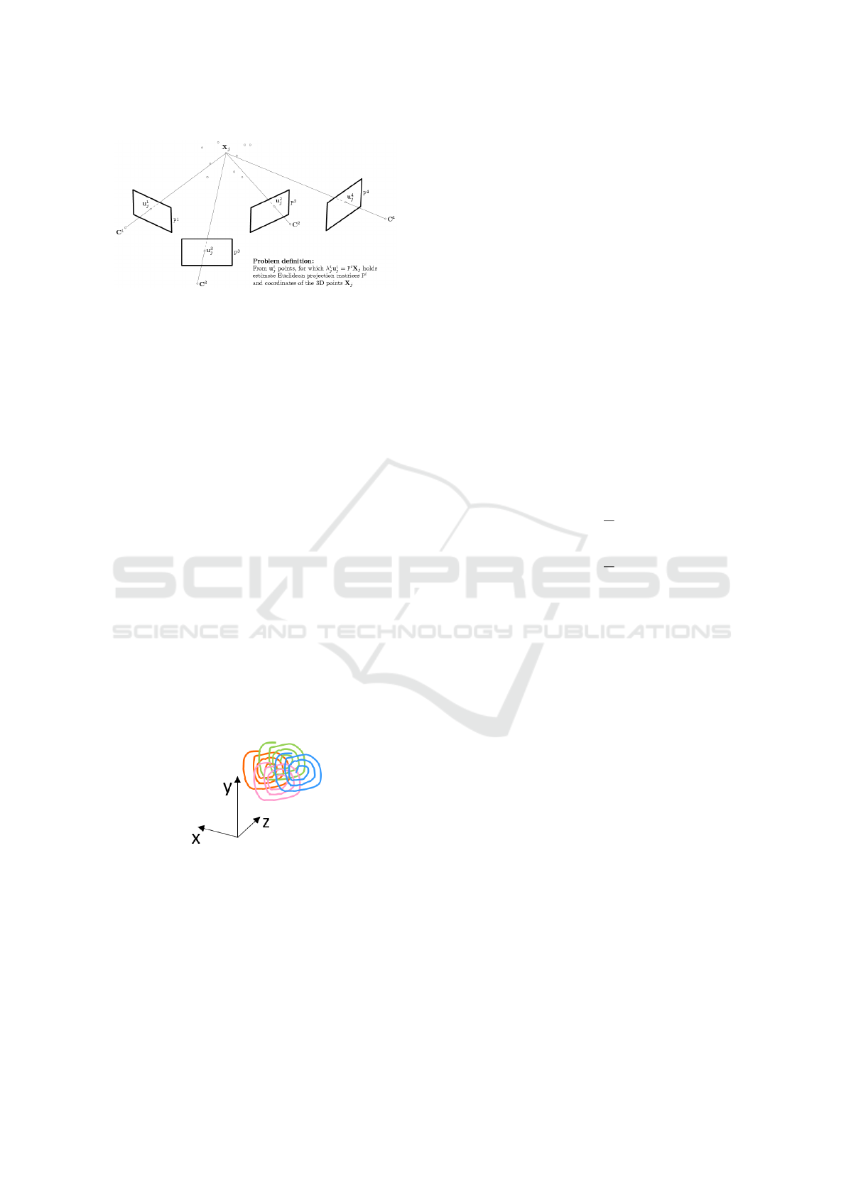
Figure 3: Multi-Camera calibration problem (Svoboda
et al., 2005).
the other hand, based on the approach described in
(Svoboda et al., 2005), where a small and easily de-
tectable bright spot is used to create a virtual calibra-
tion object. This bright spot is simultaneously visible
in all cameras avoiding the occurrence of occlusion.
Since the cameras are synchronized, the user has only
to wave the light through the working volume, there-
fore generating the required data. The remaining cal-
ibration procedure is fully automatic. The bright spot
projections are detected independently in each RGB
camera, so the correspondences are established by the
time stamps. Each detected point is also mapped into
the depth image. Before starting to generate the 3D
trajectory for calibration, the environment illumina-
tion is dimmed and the user can adjust the brightness
threshold for pointer detection and tracking. As a re-
sult, the detection of the light spot both in the RGB
image and in the infrared images (depth) is facilitated
and robust. The pointer location in the RGB image is
converted to the corresponding location in the depth
image. From the depth image, the 3D position of the
pointer (relative to the camera) was estimated. Figure
4 illustrates the four 3D trajectories, each one of them
regarding one specific camera.
Figure 4: Illustration of 3D trajectories for extrinsic calibra-
tion.
These trajectories are then filtered to remove out-
liers. The resulting filtered 3D points of each trajec-
tory are then used to estimate the relative orientations
and translations between cameras.
3.3 Finding Optimal Rotation and
Translation between Corresponding
3D Points
The optimal rigid 3D registration problem can be
characterized, according to (Arun et al., 1987) with:
RA +t = B, (3)
for noise-free data. Since the data is noisy, the least-
squares error is minimized by:
err =
N
∑
i=1
||RA
i
+t −B
i
||
2
, (4)
where A and B are sets of 3D points with known cor-
respondences. R is a 3 × 3 rotation matrix and t is the
3 × 1 translation vector.
To estimate the optimal rigid transformation, both
point clouds are centered at the origins of their co-
ordinate systems. Therefore, the centroids of both
datasets are first estimated:
centroid
A
=
1
N
N
∑
i
A
i
, (5)
centroid
B
=
1
N
N
∑
i
A
i
, (6)
where A
i
and B
i
are 3 × 1 vectors, corresponding to
the point pair i, with the coordinates of the 3D points,
i.e., [X, Y, Z]
T
.
To find the optimal rotation, we first re-center both
datasets so that both centroids are at origin. This re-
moves the translation component, leaving only the
rotation to estimate. The rotation is estimated using
the SVD method by Arun, performed on the point-set
cross-covariance matrix given by (Kanatani, 1994):
H = (A − centroid
A
)(B − centroid
B
)
T
, (7)
[U, S, V ] = SV D(H), (8)
R = VU
T
, (9)
where H is the point-set cross-covariance matrix and
A − centroid
A
is an operation that subtracts each col-
umn in A by centroid
A
. When finding the rotation
matrix, we have to take into account the case of the re-
flection matrix. That is, sometimes, the SVD method
returns this reflection matrix, which is numerically
correct but is nonsense. This is addressed by check-
ing the determinant of R and checking if it is negative
(-1). If it is, then the 3rd column of V is multiplied by
-1.
3D Reconstruction of Deformable Objects from RGB-D Cameras: An Omnidirectional Inward-facing Multi-camera System
547
After the rotation matrix is found, we estimate t
using the initial equation (3) RA + t = B but using the
centroids:
R × centroid
A
+t = centroid
B
, (10)
t = centroid
B
− R × centroid
A
. (11)
3.4 Evaluation of the Calibration
Using the data acquired as previously described, the
estimation of the relative rotation matrices and rel-
ative translation vectors can be performed. Since
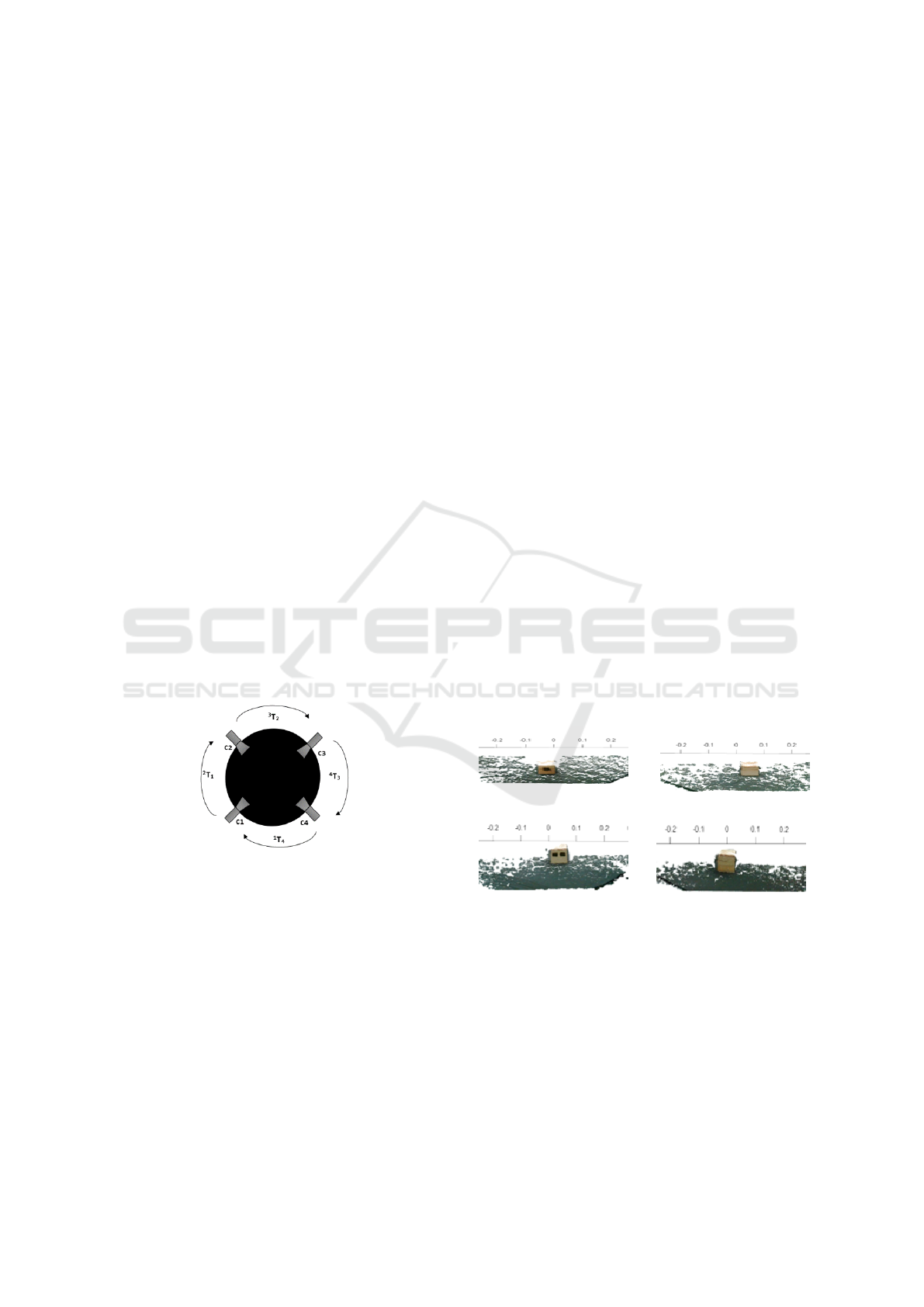
we are dealing with an omnidirectional system (Fig-
ure 5), a relative simple criterion can be applied to
estimate the overall estimation error. Assume that
T
i
j
=
R
i
j
t
i
j
0
1×3
1
represents the coordinate transfor-
mation from coordinate system i to coordinate system
j. Then, in the specific case of four coordinate sys-
tems the following condition holds:
T
2
1
.T
3
2
.T
4
3
.T
1
4
= I
4×4
(12)
This condition can be used to obtain an estimation
of the overall error in the four coordinate transforma-
tions. In general the errors obtained are small, with
the overall translation error smaller than 5% of the
distance between consecutive images. Errors in each
coordinate transformation can be minimized by using
the above error criterion in a global optimization pro-
cedure.
Figure 5: Schematic diagram representing the transforma-
tions between cameras.
4 RECONSTRUCTION
The reconstruction of a deformable object is possi-
ble since we have a synchronous acquisition system
of RGBD data and the relative positions and orienta-
tions of the cameras are known. These transforma-
tions allow us to combine the four point clouds. The
coordinate system of one of the cameras is used as a
reference coordinate system.
Since the visual fields of adjacent cameras over-
lap, duplicated points occur in the omnidirectional
point cloud. This can lead to a non-homogeneous re-
construction. To overcome this issue, the omnidirec-
tional merged point cloud is filtered using the Vox-
elGrid filter from PCL library. The VoxelGrid filter
downsamples the point cloud by taking a spatial aver-
age of the points in the cloud confined by each voxel.
The set of points which lie within the bounds of a
voxel are assigned to that voxel and are statistically
combined into one output point.
In this paper, diverse examples of object recon-
struction are presented. Firstly, we analyze the re-
constructions of a small wooden box and of a shoe
with a mold—two different objects in terms of shape,
material and color. Then, we reconstruct two white
polystyrene spheres with different radius. For the re-
construction of the spheres, in an attempt to mitigate
the noise involving the object, three acquisitions of
each camera were used to generate a mean point cloud
for the respective camera. The four mean point clouds
(corresponding to the four cameras) are then trans-
formed and filtered in one merged point cloud, simi-
lar to the previous reconstructions. Finally, the recon-
struction of a deformable object is presented, a hippo
balloon, in different stages of emptying.
4.1 Reconstruction of a Wooden Box
and a Shoe
The omnidirectional system synchronously acquired
RGB-D data viewed by each camera pointed at the
box. The different views taken at the same timestamp
of the wooden box are shown in Figure 6.
Figure 6: The four different views of the wooden box.
Figures 7 and 8 show the reconstruction of the
wooden box in different perspectives. We can notice
some noise around the corners of the box and also the
lack of sharpness of the upper face.
The shoe, unlike the box, is very curved and made
of a much brighter material. The different views of
the shoe taken at the same timestamp are in Figure 9.
In the shoe reconstructions, presented in Figures
10 and 11, it is possible to observe that, since it has
no corners, there is not as much noise as in the case
VISAPP 2021 - 16th International Conference on Computer Vision Theory and Applications
548
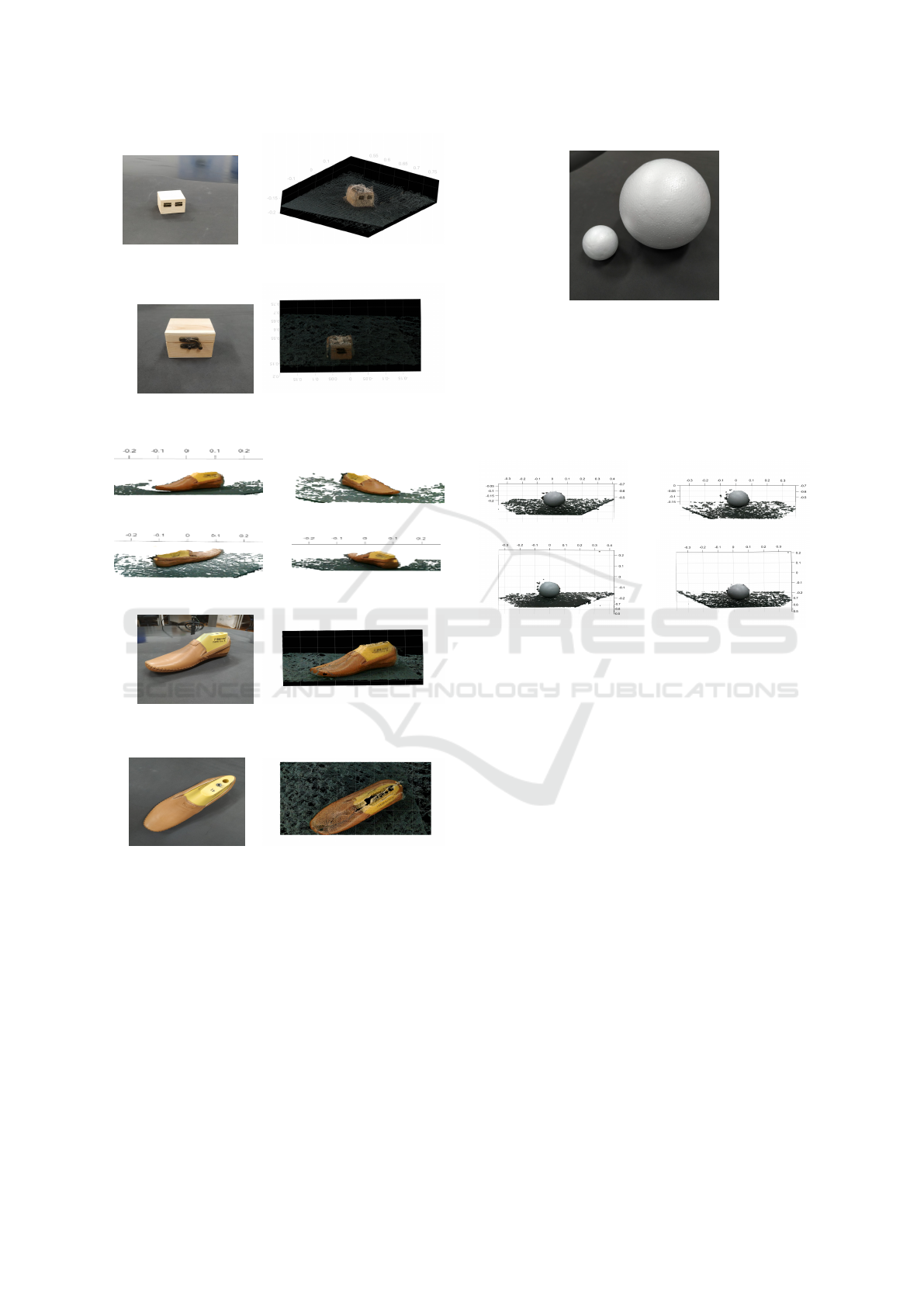
Figure 7: Real box on the left and reconstructed box on the
right: first perspective view.
Figure 8: Real box on the left and reconstructed box on the
right: second perspective view.
Figure 9: The four different views of the shoe.
Figure 10: Real shoe on the left and reconstructed shoe on
the right: first perspective view.
Figure 11: Real shoe on the left and reconstructed shoe on
the right: second perspective view.
of the box. On the other hand, we have some holes,
well visible in Figure 11, resulting from specular re-
flections.
4.2 Reconstruction of Two White
Polystyrene Spheres
The two spheres used for reconstruction are made
of white polystyrene and have a very soft surface.
The smaller sphere has approximately 3cm of radius,
while the bigger has approximately 7.5cm. The two
spheres can be seen in Figure 12.
Figure 12: Picture of the two spheres. The smaller sphere
(3cm radius) on the left and the bigger (7.5cm radius) on the
right side.
As mentioned before, for the reconstruction of the
spheres three point clouds from each camera were ac-
quired, with the aim of generating an average point
cloud. In Figure 13 the average point clouds for the
biggest sphere are presented.
Figure 13: The four different views of the sphere.
Similar to the other reconstructions, these views
are then used to build the omnidirectional point cloud.
In order to analyze the quality of the reconstructions,
for both, the 3cm radius and the 7,5cm radius sphere,
the approximated model of the spheres was estimated.
The parameters of the models were obtained using a
robust estimator, the M-estimator SAmple Consen-
sus (MSAC) algorithm (Torr and Zisserman, 2000).
This RANSAC variation is based on the following
steps: drawing randomly a minimal sample set; esti-
mating the model and then evaluating the model. This
process is repeated until the last iteration that corre-
sponds to the best model.
In Figures 14 and 15, we can view the estimated
model of the spheres fitting the point clouds of the
real spheres.
To analyze the reconstruction of the spheres we
used the mean error, that is, the average of the dis-
tances from the inliers points (points belonging to the
point cloud that were used to estimate the paramet-
ric model of the sphere) to the surface of the sphere
generated by the parametric model. In table 2, the av-
erage errors for the two spheres are presented for four
cases namely: the reconstruction made with only one
acquisition per camera, 1
st
acquisition, 2
nd
acquisi-
tion and 3
rd
acquisition and the reconstruction made
3D Reconstruction of Deformable Objects from RGB-D Cameras: An Omnidirectional Inward-facing Multi-camera System
549
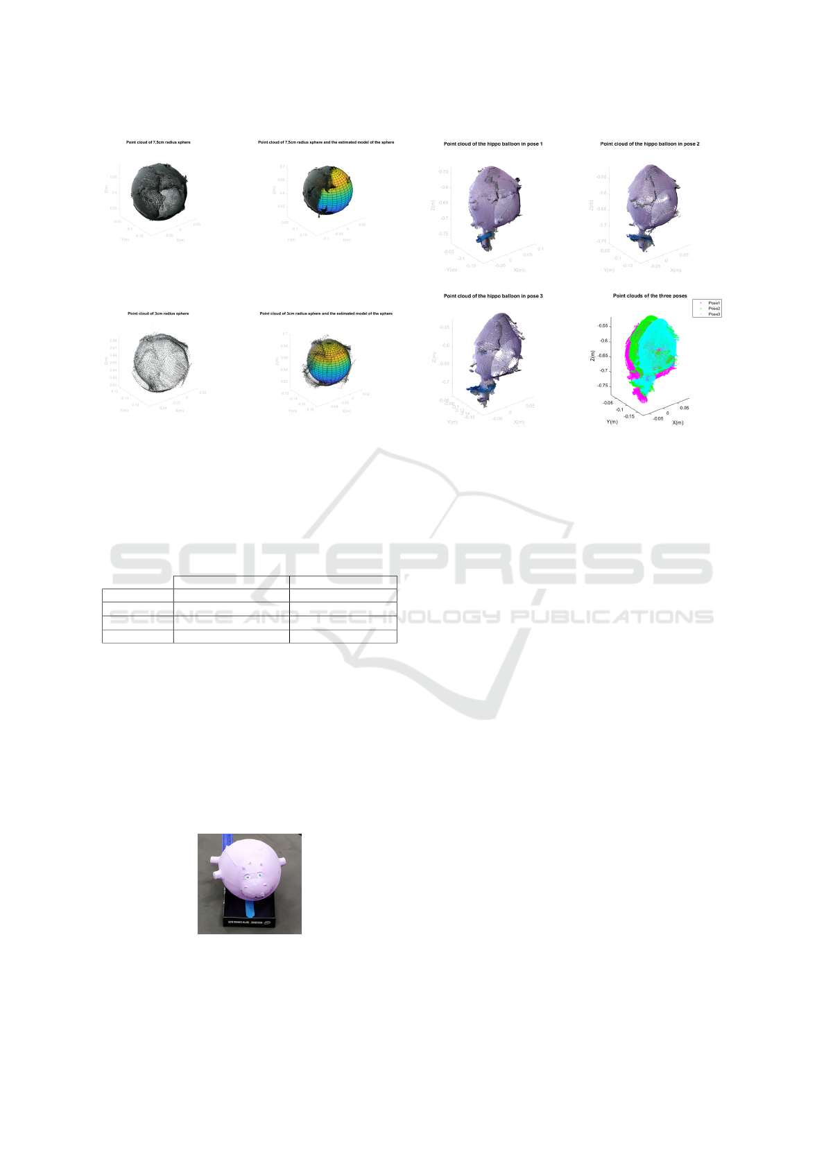
Figure 14: On the left side we have the point cloud of the
7,5cm radius sphere and on the right side, the point cloud
and the plot of the sphere model.
Figure 15: On the left side we have the point cloud of the
3cm radius sphere and on the right side, the point cloud and
the plot of the sphere model.
with the mean point clouds. The smallest average er-
ror is obtained for the reconstruction performed with
the mean point clouds.
Table 2: The mean errors obtained for the different esti-
mates of the parametric models.
Sphere of radius 7.5cm Sphere of radius 3cm
1
st
acq. 0.0034m 0.0020m
2
nd
acq. 0.0029m 0.0020m
3
rd
acq. 0.0033m 0.0021m
Mean of acq. 0.0021m 0.0017m
4.3 Reconstruction of a Hippo Balloon
Deforming
For the reconstruction of the balloon in Figure 16,
point clouds were acquired during its emptying.
The balloon was reconstructed in three different
stages/time instants, considering that in each stage,
the images from each camera are synchronized. The
reconstructions are shown in Figure 17, where a plot
with the three point clouds together is also presented.
Figure 16: Picture of the hippo-shaped balloon.
Figure 17: The first three plots show the hippo balloon’s
reconstructions in three different sequential phases of the
emptying. The fourth image illustrates the three point
clouds, being notorious the deformation occurring with the
emptying.
5 CONCLUSION
This paper describes a system designed to acquire
synchronized 3D omnidirectional images of objects.
That allows for the 3D reconstruction of objects that
are articulated or deformable. The experimental re-
sults show that specular surfaces as well as sharp cor-
ners do not yield good quality reconstructions. Since
no controlled illumination is used in the system, we
plan to add an illumination system to improve the re-
construction quality. The reconstructions of spheres
allow us to conclude that the reconstructions that use
the mean of point clouds from each camera seem to
have a lower mean error relative to its sphere models,
which is an indicator that reconstruction itself is also
better. Finally, the balloon’s reconstruction shows that
this system is suitable for the reconstruction of objects
that deform.
ACKNOWLEDGEMENTS
This work was partially supported by Project COM-
MANDIA SOE2/P1/F0638, from the Interreg Sudoe
Programme, European Regional Development Fund
(ERDF), and by the Portuguese Government FCT,
project no. 006906, reference UID/EEA/00048/2013.
VISAPP 2021 - 16th International Conference on Computer Vision Theory and Applications
550

REFERENCES
Arun, K. S., Huang, T. S., and Blostein, S. D. (1987). Least-
squares fitting of two 3-d point sets. IEEE Trans-
actions on pattern analysis and machine intelligence,
(5):698–700.
Curless, B. and Levoy, M. (1996). A volumetric method for
building complex models from range images. In Pro-
ceedings of the 23rd annual conference on Computer
graphics and interactive techniques, pages 303–312.
Dai, A., Nießner, M., Zollh
¨
ofer, M., Izadi, S., and Theobalt,
C. (2017). Bundlefusion: Real-time globally consis-
tent 3d reconstruction using on-the-fly surface rein-
tegration. ACM Transactions on Graphics (ToG),
36(4):1.
Grunnet-Jepsen, A., Winer, P., Takagi, A., Sweetser, J.,
Zhao, K., Khuong, T., Nie, D., and Woodfill, J. (2018).
Using the Intel
R
RealSense TM Depth cameras
D4xx in Multi-Camera Configurations.
Innmann, M., Zollh
¨
ofer, M., Nießner, M., Theobalt, C.,
and Stamminger, M. (2016). Volumedeform: Real-
time volumetric non-rigid reconstruction. In Euro-
pean Conference on Computer Vision, pages 362–379.
Springer.
Kanatani, K.-i. (1994). Analysis of 3-d rotation fitting.
IEEE Transactions on pattern analysis and machine
intelligence, 16(5):543–549.
Matsumoto, J. and Aguilar-Rivera, M. (2018). 3DTracker-
FAB documentation.
Newcombe, R. A., Fox, D., and Seitz, S. M. (2015). Dy-
namicfusion: Reconstruction and tracking of non-
rigid scenes in real-time. In Proceedings of the IEEE
conference on computer vision and pattern recogni-
tion, pages 343–352.
Newcombe, R. A., Izadi, S., Hilliges, O., Molyneaux, D.,
Kim, D., Davison, A. J., Kohi, P., Shotton, J., Hodges,
S., and Fitzgibbon, A. (2011). Kinectfusion: Real-
time dense surface mapping and tracking. In 2011
10th IEEE International Symposium on Mixed and
Augmented Reality, pages 127–136. IEEE.
Rusinkiewicz, S., Hall-Holt, O., and Levoy, M. (2002).
Real-time 3d model acquisition. ACM Transactions
on Graphics (TOG), 21(3):438–446.
Slavcheva, M., Baust, M., Cremers, D., and Ilic, S. (2017).
Killingfusion: Non-rigid 3d reconstruction without
correspondences. In Proceedings of the IEEE Con-
ference on Computer Vision and Pattern Recognition,
pages 1386–1395.
Slavcheva, M., Baust, M., and Ilic, S. (2018). Sobolev-
fusion: 3d reconstruction of scenes undergoing free
non-rigid motion. In Proceedings of the IEEE Con-
ference on Computer Vision and Pattern Recognition,
pages 2646–2655.
Svoboda, T., Martinec, D., and Pajdla, T. (2005). A con-
venient multicamera self-calibration for virtual envi-
ronments. Presence Teleoperators Virtual Environ.,
14(4):407–422.
Torr, P. H. and Zisserman, A. (2000). Mlesac: A new ro-
bust estimator with application to estimating image
geometry. Computer vision and image understanding,
78(1):138–156.
Whelan, T., Salas-Moreno, R. F., Glocker, B., Davi-
son, A. J., and Leutenegger, S. (2016). Elasticfu-
sion: Real-time dense slam and light source estima-
tion. The International Journal of Robotics Research,
35(14):1697–1716.
Zollh
¨
ofer, M., Nießner, M., Izadi, S., Rehmann, C., Zach,
C., Fisher, M., Wu, C., Fitzgibbon, A., Loop, C.,
Theobalt, C., et al. (2014). Real-time non-rigid recon-
struction using an rgb-d camera. ACM Transactions
on Graphics (ToG), 33(4):1–12.
3D Reconstruction of Deformable Objects from RGB-D Cameras: An Omnidirectional Inward-facing Multi-camera System
551
