Machine Learning Studies of Non-coding RNAs based on Artiﬁcially

Constructed Training Data

Mirele C. S. F. Costa

1,† a

, Jo

ao Victor A. Oliveira

2 b

, Waldeyr M. C. da Silva

1,3 c

Rituparno Sen

4 d

, J

org Fallmann

4 e

, Peter F. Stadler

4,5,6,7 f

and Maria Em

ılia M. T. Walter

1,‡ g

University of Bras

ılia (UnB), Brazil

Federal Institute of Bras

ılia (IFB), Brazil

Federal Institute of Goi

as (IFG), Brazil

Bioinformatics Group, Department of Computer Science, Interdisciplinary Center for Bioinformatics,

University of Leipzig, Leipzig, Germany

German Centre for Integrative Biodiversity Research (iDiv) Halle-Jena-Leipzig, Leipzig, Germany

Max Planck Institute for Mathematics in the Sciences, Leipzig, Germany

Santa Fe Institute, Santa Fe, U.S.A.

Keywords:

Small Nucleolar RNAs (snoRNAs), Non-Coding RNA Inference, Machine Learning, Chordate Genome.

Abstract:

Machine learning (ML) methods are often used to identify members of non-coding RNA classes such as

microRNAs or snoRNAs. However, ML methods have not been successfully used for homology search tasks.

A systematic evaluation of ML in homology search requires large, controlled, and known ground truth test

sets, and thus, methods to construct large realistic artiﬁcial data sets. Here we describe a method for producing

sets of arbitrarily large and diverse snoRNA sequences based on artiﬁcial evolution. These are then used to

evaluate supervised ML methods (Support Vector Machine, Artiﬁcial Neural Network, and Random Forest) for

snoRNA detection in a chordate genome. Our results indicate that ML approaches can indeed be competitive

also for homology search.

1 INTRODUCTION

Many distinct classes of non-coding RNAs (ncRNAs)

are known, each with speciﬁc function, in turn de-

pending on their spatial structure, sequence compo-

sition and length. In this contribution we focus on

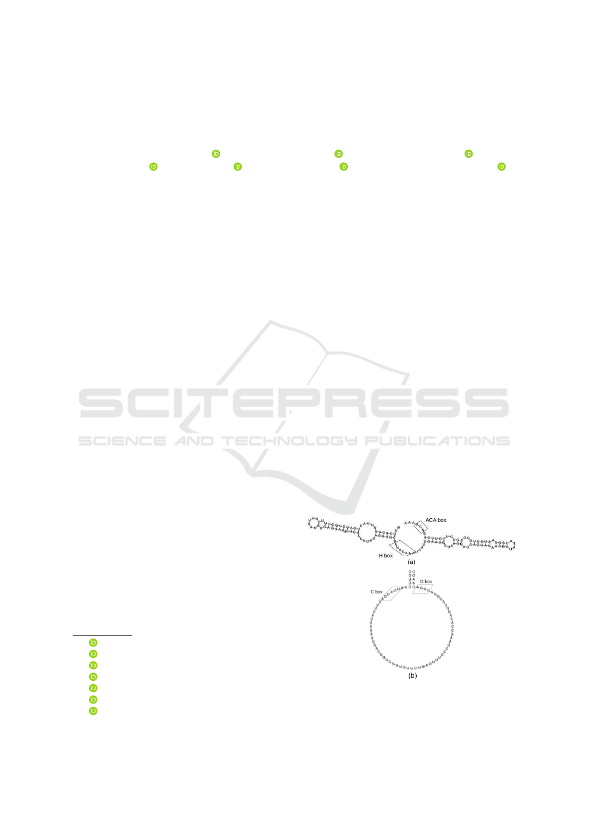
small nucleolar RNAs (snoRNAs). They form a large

class of RNAs with lengths varying from 60 to 300

nucleotides that comprises two functionally and struc-

turally distinct subclasses, the H/ACA box and C/D

box (Falaleeva and Stamm, 2013) (see Figure 1). In

animals, snoRNAs are processed from introns of both

coding and non-coding host RNAs (Bratkovi

c et al.,

2020).

https://orcid.org/0000-0002-1337-4672

https://orcid.org/0000-0003-3622-1334

https://orcid.org/0000-0002-8660-6331

https://orcid.org/0000-0001-5980-5565

https://orcid.org/0000-0002-4573-9939

https://orcid.org/0000-0002-5016-5191

https://orcid.org/0000-0001-6822-931X

There are two fundamentally different methods

to identify ncRNAs in genomic data: (1) Homol-

ogy search utilizes sequence similarity to a speciﬁc

Figure 1: Two-Dimensional structure of (a) H/ACA box

snoRNA; and (b) C/D box snoRNA (de Araujo Oliveira

et al., 2016).

176

Costa, M., Oliveira, J., C. da Silva, W., Sen, R., Fallmann, J., Stadler, P. and Walter, M.

Machine Learning Studies of Non-coding RNAs based on Artiﬁcially Constructed Training Data.

DOI: 10.5220/0010346001760183

In Proceedings of the 14th International Joint Conference on Biomedical Engineering Systems and Technologies (BIOSTEC 2021) - Volume 3: BIOINFORMATICS, pages 176-183

ISBN: 978-989-758-490-9

query sequence. Since structure dictates function of

many RNAs, their spatial structures are often bet-

ter conserved than their sequences. Thus, homol-

ogy search methods for ncRNAs usually also take

structural similarity into account. Tools such as

infernal (Nawrocki and Eddy, 2013) indeed achieve

substantial improvements compared to sequence-only

methods such as Blast (Altschul et al., 1990), see

e.g. (Bartschat et al., 2014). However, by construc-

tion, only homologs of known ncRNAs can be found.

(2) Some ncRNAs, including transferRNAs, microR-

NAs, and snoRNAs, belong to larger families that

share both function and biogenesis and are conse-

quently recognizable by a set of characteristic se-

quence and structure features. The identiﬁcation of

members of an RNA class is a classiﬁcation prob-

lem that is typically solved by machine learning meth-

ods (Zhang et al., 2017; Barber, 2012; Zhang and Ra-

japakse, 2009). SnoReport 2.0 (de Araujo Oliveira

et al., 2016) implements such a classiﬁer for snoR-

NAs. It extracts a combination of sequence and sec-

ondary features, the latter predicted by thermody-

namic folding (Lorenz et al., 2011), from a query se-

quence and employs a support vector machine (SVM)

for classiﬁcation into the two main classes of snoR-

NAs: the H/ACA box and the C/D box. SnoReport

2.0 can be used to scan large DNA sequences, using

characteristic sequence and structure motifs to iden-

tify candidates that are passed to the SVM classi-

ﬁer. Similarly, classiﬁers for miRNAs start from a

predicted precursor hairpin. This makes the classi-

ﬁcation problem fairly simple since the task merely

distinguishes whether the input sequence is exactly a

class member.

A closely related, but apparently much more difﬁ-

cult machine learning problem is to ask whether or not

a given sequence of ﬁxed length contains a ncRNA of

a given class. An efﬁcient solution to this version of

the ncRNA classiﬁcation problem would provide an

alternative to homology search for large evolutionary

distance, where sequence similarity comes close to or

even falls below the detection limit. Anecdotal reports

on attempts to use machine learning for this task, e.g.,

(Waldl et al., 2018), however, have been discourag-

ing – albeit this may be a consequence of very small

training sets. A more systematic investigation into

the feasibility of machine learning as an alternative

to direct sequence comparison requires training and

test sets that are large and diverse enough. Further-

more, they have to cover a wide range of evolutionary

distances from closely related sequences to homologs

that have diverged beyond the detection limit for se-

quence alignment methods.

In this contribution, we present a method to gen-

erate in principle an arbitrarily large and diverse data

set of artiﬁcial ncRNAs, using snoRNAs as an exam-

ple. The key idea is to simulate the evolution of the

ncRNAs along a real or randomly generated phyloge-

netic tree, using a classiﬁer for the ncRNAs of inter-

ests, here snoReport 2.0, to model selection. That

is, mutations are only accepted if they pass the clas-

siﬁer. The procedure thus “breeds” snoRNAs with

increasingly divergent sequences that are still recog-

nizable as snoRNAs. The artiﬁcial ncRNAs can then

be inserted into background genomes to produce re-

alistic data with perfectly-known ground truth to train

and benchmark homology search methods. Here we

consider Support Vector Machines (SVMs), Random

Forests (RFs), and artiﬁcial neural networks (ANNs)

as classiﬁcation methods.

2 METHODS

We start in Section Initial Data with a description of

the biological data that we use as starting point and for

evaluation purposes. We then describe construction

of an artiﬁcial snoRNA data set (”Breeding” Artiﬁ-

cial snoRNAs). The third part of this section (Feature

Extraction) summarizes the features used to evaluate

de ML methods. Finally, we provide a detailed evalu-

ation of ML approaches versus direct sequence com-

parison. On the top level, the workﬂow starting with

the initially acquired data can be subdivided into six

stages, which are also presented in ﬁgure 2:

1. Run snoReport 2.0 over the selected intron se-

quences to identify snoRNAs and their corre-

sponding C/D or H/ACA boxes.

2. Choose randomly representative snoRNA se-

quences from snoReport 2.0 output to apply

mutations;

3. Build mutation tree using the snoReport 2.0

output sequences composing sets with cumulative

percentage of mutations;

4. Extract features for each sequence, considering

the positive and negative sets obtained from the

mutation tree;

5. Construct datasets for ML algorithms with the

same number of instances for the positive (1) and

negative (0) sets.

6. Execute ML algorithms and analyze their results.

2.1 Initial Data

The source data used in the experiments was extracted

from the marine species Ciona intestinalis, obtained

Machine Learning Studies of Non-coding RNAs based on Artiﬁcially Constructed Training Data

177

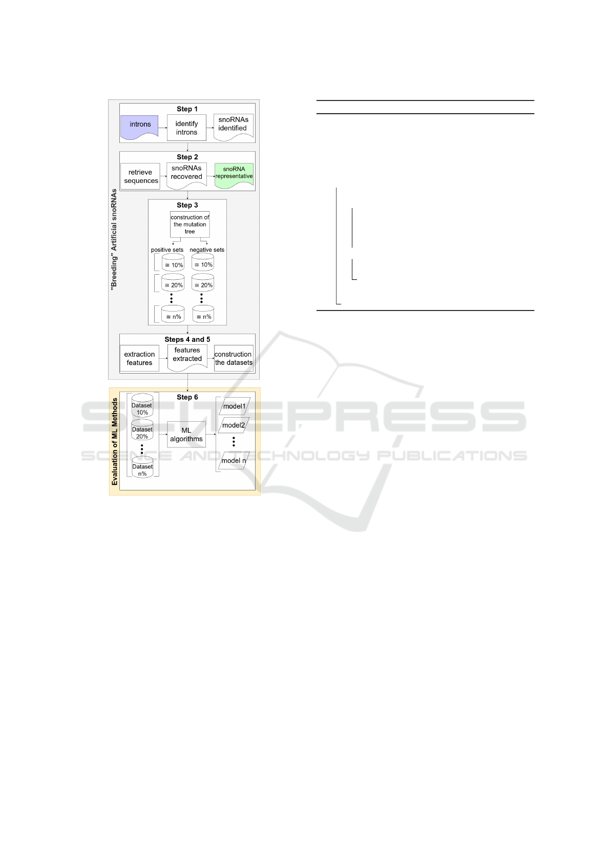
Figure 2: Summary of the steps to build the dataset and

analyze the machine learning methods.

from the National Center for Biotechnology Informa-

tion (NCBI). We retrieved the genome and transcript

sequences in fasta format, and the genome annota-

tion in a GFF3 format. C. intestinalis is an attrac-

tive model for studying chordate origins and evolu-

tion since it has a compact genome, which is advanta-

geous for developmental evolutionary studies (Satoh,

2003). We used Blastn (Altschul et al., 1990) to lo-

cate the known snoRNA sequences from C. intesti-

nalis in the annotated intronic sequences, which were

retrieved using GFF-Ex (Rastogi and Gupta, 2014). A

cut-off of 80% sequence identity was employed. This

resulted in one H/ACA box snoRNA and two C/D box

snoRNAs, which served as starting points for our sim-

ulations.

Algorithm 1: Construction of the mutation tree.

Data: s// a snoRNA sequence intron// the

intron containing the snoRNA

sequence

Result: T // a mutation tree

1 mutate s: sMutated

2 replace s by a sMutated into the intron

3 if intron has a snoRNA then

4 if sMutated is identiﬁed as snoRNA in the same

locus of the original one then

5 sMutated is inserted into T , to be

successively mutated;

6 sMutated is stored in the positive set

corresponding to the tree level;

7 else

8 sMutated is not inserted into T and is stored

in a separate set;

9 sMutated is not inserted into T and is stored in

the negative set;

2.2 ”Breeding” Artiﬁcial snoRNAs

SnoReport 2.0 was used to identify snoRNA se-

quences and their corresponding C/D box or H/ACA

box classes in the carefully selected intron sequences

as described in subsection 2.1 (Fig 2-Step 1). From

those sequences, two representatives were chosen to

generate the mutation trees, one C/D box snoRNA

and one H/ACA box snoRNA (Fig 2-Step 2). The

total length of the intron and of the original snoRNA

are 833 and 96, for C/D box, and 173 and 1,577, for

H/ACA box, respectively. Algorithm 1 describes the

construction of the mutation tree and thus of the artiﬁ-

cial snoRNAs. These are then used to deﬁne positive

and negative sets for the classiﬁcation task (Fig 2-Step

3).

The root of the tree corresponds to one of the

representative snoRNA sequences s described above.

In each step, mutations (substitutions, deletions, and

insertions) are applied to s. The resulting mutated

sequence sMutated is then re-inserted into the in-

tronic sequences. We deﬁne sMutated as a synthetic

snoRNA, i.e., as a true positive, if it is recognized in

this context as a snoRNA by snoReport 2.0. Muta-

tion trees are constructed independently for each ini-

tial snoRNA. In each level of the tree we train at most

N sequences. The mutation process mimics a popu-

lation of ﬁxed size with N = 3000 sequences for C/D

box and N = 2000 for H/ACA box to limit the compu-

tational resources. In order to obtain balanced trees,

the sequence to be mutated is chosen at random from

this population. The nodes of mutation tree are gener-

ated with 10 children. The positive set consists of the

mutated sequences inserted into the introns that are

still recognized as snoRNAs. As the mutations are

BIOINFORMATICS 2021 - 12th International Conference on Bioinformatics Models, Methods and Algorithms

178

Figure 3: (a) Example of a mutation tree with 3 children and

a maximum of 5 nodes per level. The sequences shown in

the tree are in the positive set. (b) Example of a negative set

(sequences are not in the tree) and a positive set with 10%

mutated positions (10 nucleotide length sequence).

cumulative, the positive set comprises of sequences

with approximately the same percentage of mutations.

For example 10%, 20 %, 30%, 40% and 50% of po-

sitions mutated relative to the representative snoRNA

sequence. The negative set is formed by the mutated

sequences sMutated that could no longer be identi-

ﬁed as snoRNAs. Each negative set is composed of

sequences with the same mutation percentage, simi-

lar to the positive set. For a better understanding of

the positive and negative sets, we illustrate an exam-

ple with 10% of mutated positions in Figure 3.

2.3 Feature Extraction

We extracted features for each sequence of positive

and negative sets obtained from the mutation tree.

(Fig 2-Step 4). The following features are extracted

from the C/D box sequences: mfe (Minimum Free En-

ergy of the secondary structure without constraints);

mfeC (MFE of the secondary structure with con-

straints); E

avg

(MFE average); E

stdv

(MFE standard

deviation); ls (length of the terminal stem); Dcd (dis-

tance between C and D boxes); C

score

(score of the

C box); D

score

(score of the D box); GC (GC con-

tent); zscore (z-score obtained by RNAz 2.0 (Gruber

et al., 2010)); bpStem (number of base pairs on the

terminal stem); lu5 (number of unpaired nucleotides

inside the stem before C box); lu3 (number of un-

paired nucleotides inside the stem after D box); stemU

npCbox (number of unpaired nucleotides between the

stem and the C box); stemU npDbox (number of un-

paired nucleotides between the D box and the stem).

The following features are extracted from the

H/ACA box sequences with snoReport 2.0: mfeC

(MFE of the secondary structure with constraints);

AC, GU, GC (AC, GU and GC content); zscore (zs-

core computed by RNAz); Hscore (score of the H

Table 1: C/d box and H/ACA box.

snoRNA Type tree N n(1) n(0)

substitution 3000 2574 2574

C/D insertion 3000 1795 1795

deletion 3000 2232 2232

substitution 2000 1835 1835

H/ACA insertion 2000 1009 1009

deletion 2000 1664 1664

box); ACAscore (score of the ACA box); LseqSize

(number of nucleotides before the H box); RseqSize

(number of nucleotides between H and ACA boxes);

LloopSC (lenght of the loop, where we ﬁnd the pocket

region containing the target region, near to the H box);

RloopSC (length of the loop, where we ﬁnd the pocket

region containing the target region, more close to the

ACA box); LloopY C (symmetry of the loop contain-

ing the pocket region near to the H box); RloopY

C (symmetry of the loop containing the pocket re-

gion near to the ACA box); LloopSym (symmetry of

all loops before H box); RloopSym (symmetry of all

loops before ACA box).

The datasets are ﬁles in Comma-separated values

(CSV) format composed of the same number of in-

stances extracted from the positive (1) and negative

(0) sets. Since different sequence may produce the

same feature values. Therefore, duplicated feature

vectors are removed from both the positive and nega-

tive set. For each mutation tree, we verify the pos-

itive set with the least number n of instances. We

constructed datasets comprising different numbers n

of sequences. For a given n, we randomly chose n in-

stances from the positive and negative sets according

to the percentage of mutation. Example, the dataset

with 10% mutation is composed of n instances of the

positive set with 10% mutation and n instances of the

negative set with approximately 10% mutation.

Normalization by linear interpolation (Gold-

schmidt and Passos, 2005) was applied to the features

extracted from the sequences of the positive and nega-

tive sets, i.e., feature values were transformed accord-

ing to x

= (x − x

min

)/(x

max

− x

min

). This preserves

proportional distances between normalized data and

the distances between the original data (Fig 2-Step 5).

For both C/D box and H/ACA box snoRNAs we gen-

erated three mutation trees, one for each of the types

of mutation (substitution, insertion, deletion). Table 1

list, for C/D box and H/ACA box, respectively, the

number N of sequences of the positive sets (Fig 2 -

Step 3), the number n(1) of feature vectors extracted

from the N sequences of the positive set, the number

n(0) of feature vectors extracted from the sequences

of the negative set (Fig 2 - Step 4).

Machine Learning Studies of Non-coding RNAs based on Artiﬁcially Constructed Training Data

179

2.4 Evaluation of Machine Learning

Methods

Our goal is to evaluate the use of ML methods in

the context of ncRNA homology search. To this

end, we apply three ML algorithms, SVM (Rus-

sell and Norvig, 2010), Artiﬁcial Neural Net-

work (ANN) (Haykin, 1999) and Random For-

est (RF) (Breiman, 2001). These methods were

chosen since they have been extensively used for

ncRNA classiﬁcation tasks (Georgakilas et al., 2020;

Achawanantakun et al., 2015). The evaluation of

SVM is not entirely fair in comparison to the other

methods, since snoReport 2.0 also uses an SVM,

albeit trained on different data and embedded in ad-

ditional ﬁlters. It still provides valuable informa-

tion on the limitations of the ML approaches. We

use Jupyter-notebook to implement the supervised

learning algorithms, language packages in Python,

Keras (Gulli and Pal, 2017) and Scikit-learn (Pe-

dregosa et al., 2011). For SVM, we use the Ra-

dial basis function kernel (RBF), while for ANN we

use the sequential model of neural network, with

three layers of the Dense type, and, ﬁnally, for RF,

we use one hundred decision trees built using the

Bagging technique (by default). We tested all the

datasets on the ML algorithms, with 10-fold cross-

validation (Fig 2-Step 6). To evaluate ML algorithms,

we report the following evaluation metrics: Area Un-

der The Curve (AUC), Matthews Correlation Coefﬁ-

cient (MCC), Recall, Precision and Receiver Operat-

ing Characteristic Curve (ROC curve).

3 RESULTS AND DISCUSSION

We executed Blastn with default scoring using as

queries, the biological snoRNA sequences (tree roots)

and as databases each of the positive sets generated by

the mutation trees (with mutation rates of 10%, 20%,

30%, 40% and 50%, and N = 3, 000 for C/D box and

N = 2,000 for the H/ACA box). The sequences, the

original snoRNAs and the mutated ones, were tested

inside the introns, and also considering only the se-

quences themselves. To quantify the success of this

sequence-based homology search, we computed an

average hit rate, M := S/N, where S is the number

of aligned sequences and N is the total number of se-

quences (query ﬁle length).

With the snoRNAs inside the intron, Blastn al-

ways found matches, so in this case M = 100%. How-

ever, in most cases these did not match only the target

snoRNA but were spurious hits elsewhere in the in-

tron. Disregarding the decoy sequences, we obtained

essentially the same results with Blastn, independent

of the mutation model.

With the snoRNAs themselves, Blastn found

matches only for 10% and 20%, all of them with an

e-value ≤ 0.01. For substitutions, as example, we ob-

tained M = 18.9% and M = 0.5% for C/D box snoR-

NAs, and M = 73.6% and M = 2.9% for H/ACA box

snoRNAs at 10% and 20% mutation rate, respectively.

At even higher level of sequence divergence, Blastn

did not recover any snoRNA. We therefore have con-

structed a homology search problem that is very dif-

ﬁcult for Blastn, the most widely used tool for this

task. These results certainly could be improved by

adapting Blastn for distance homologies or by using

Hidden Markov Models (HMMs) that use a pattern

instead of a single sequence as query. We did not pur-

sue this, since our main interest is to demonstrate that

ML algorithms are capable of handling such a difﬁ-

cult homology search problem.

3.1 C/D Box

We performed experiments for each mutation tree

(substitution, insertion and deletion). From these, we

chose substitution and insertion to discuss results in

more detail.

Substitution. Table 2 shows the results of the three

ML algorithms for the substitution experiment.

The ANN and SVM showed decreasing values for

all evaluation metrics. With 10% of ANN mutation

they obtained MCC = 98.84(%) and SVM MCC =

96.97(%), with 50% of mutation ANN and SVM they

obtained MCC = 63.36(%) and MCC = 44.44(%), re-

spectively. We can see in Fig 4 the ROC curves of

these two classiﬁers, the models achieved a good mea-

Table 2: Results ML algorithms for substitution with all fea-

tures C/D box: Area Under The Curve (AUC), Matthews

Correlation Coefﬁcient (MCC), Recall (R) and Precision

(P).

ML Datasets AUC(%) MCC(%) R(%) P(%)

10(%) 99.42 98.84 99.18 99.65

20(%) 97.79 95.64 96.16 99.40

ANN 30(%) 93.93 88.65 88.35 99.43

40(%) 93.96 88.55 90.17 97.56

50(%) 80.32 63.36 72.27 86.16

10(%) 98.47 96.97 97.71 99.21

20(%) 96.14 92.35 94.49 97.71

SVM 30(%) 93.55 87.31 93.55 93.55

40(%) 88.53 77.45 89.59 87.72

50(%) 71.47 44.44 77.90 69.03

10(%) 77.21 56.61 57.32 95.23

20(%) 91.19 82.96 83.30 98.89

RF 30(%) 72.98 47.40 47.38 97.13

40(%) 93.03 86.52 90.80 95.04

50(%) 78.40 57.63 71.15 83.23

BIOINFORMATICS 2021 - 12th International Conference on Bioinformatics Models, Methods and Algorithms

180

Figure 4: ROC curves of the datasets with 10%, 20%, 40%

and 50% of mutations, for substitution, with all features.

sure of separability for datasets with 10%, 20%, 30%

and 40% mutation. However, for datasets with 50%

mutation, they showed less capacity for class separa-

tion. RF obtained good results in all evaluation met-

rics for 20% and 40% mutation. The other datasets

10%, 30% and 50% did not achieve good results, pre-

diction with MCC = 56.61(%), MCC = 47.40(%) and

MCC = 57.63(%) respectively.

In order to investigate cases where biological char-

acteristics are not known, we also tested the ML algo-

rithms with a reduced number of features, in this case

- zscore, ls, Dcd, GC, lu5, and lu3. The three classi-

ﬁers did not achieve good results in all datasets, or the

models did not show a good predictive capacity.

Insertion. Table 3 shows the results of the three ML

algorithms for the insertion experiment.

The SVM classiﬁer presented a good prediction in

all datasets, with 10% of mutations AUC = 97.71%,

and 50% of mutations, AUC = 94.01%, as shown by

Table 3: Results ML algorithms for insertion with all fea-

tures C/D box: Area Under The Curve (AUC), Matthews

Correlation Coefﬁcient (MCC), Recall (R) and Precision

(P).

ML Datasets AUC(%) MCC(%) R(%) P(%)

10(%) 82.17 65.42 64.87 99.23

20(%) 81.70 68.21 63.77 99.48

ANN 30(%) 78.55 59.77 57.41 99.52

40(%) 91.73 84.58 84.97 98.26

50(%) 92.26 85.20 86.97 97.26

10(%) 97.71 95.53 95.94 99.48

20(%) 96.71 93.58 94.16 99.24

SVM 30(%) 93.76 88.17 88.75 98.64

40(%) 94.27 88.97 89.64 98.77

50(%) 94.01 88.48 89.37 98.53

10(%) 53.83 9.61 9.69 82.86

20(%) 49.3 -3.63 1.17 31.34

RF 30(%) 49.72 0.53 2.67 45.28

40(%) 50.11 1.16 0.56 62.50

50(%) 54.3 4.88 9.52 90.96

Figure 5: ROC curves of the datasets with 10%, 20%, 40%

and 50% of mutations, for insertion with all features.

the ROC curves in Fig 5. The RF classiﬁer model

did not achieve class separation capability in all the

datasets, with 10% of mutations, AUC = 53.83%, and

50% of mutations AUC = 54.30%, as shown in the

ROC curves in Fig 5. The ANN classiﬁer presents a

good prediction for the datasets, with 40% of muta-

tions, AUC = 91.73% and 50%, AUC = 92.26%, as

shown by the ROC curves in Fig 5. In this experi-

ment, the insertion mutation may have evidenced C/D

box characteristics.

We also tested a reduced number of features for in-

sertion, in this case zscore, ls, Dcd, GC, lu5, and lu3.

The ANN and SVM classiﬁers achieved lower perfor-

mance but still remained functional. As with substi-

tution, these two experiments with insertion showed

that the set of features is very important for predict-

ing the C/D box by ML classiﬁers. If relevant biolog-

ical characteristics are not known, the performance of

the classiﬁers deteriorates, in particular for the more

distant homologs.

3.2 H/ACA Box

We performed our experiments for each mutation

tree(substitution, insertion and deletion). From our

experiments, we choose substitution and insertion to

discuss results in more detail.

Substitution. Table 4 shows the results of the three

ML algorithms for the substitution experiment.

The SVM and RF classiﬁers showed decreasing

values for all evaluation metrics table 4. With 10%

of mutations, ANN obtained AUC = 74.20%, SVM

AUC = 67.76% and RF AUC = 62.03%. With 50%

mutation, the results were even lower, ANN, SVM

and RF obtained AUC = 59.08%, AUC = 61.36% and

AUC = 50.57% respectively. We can see the corre-

sponding ROC curves in Fig 6.

For H/ACA box, in order to investigate cases

Machine Learning Studies of Non-coding RNAs based on Artiﬁcially Constructed Training Data

181

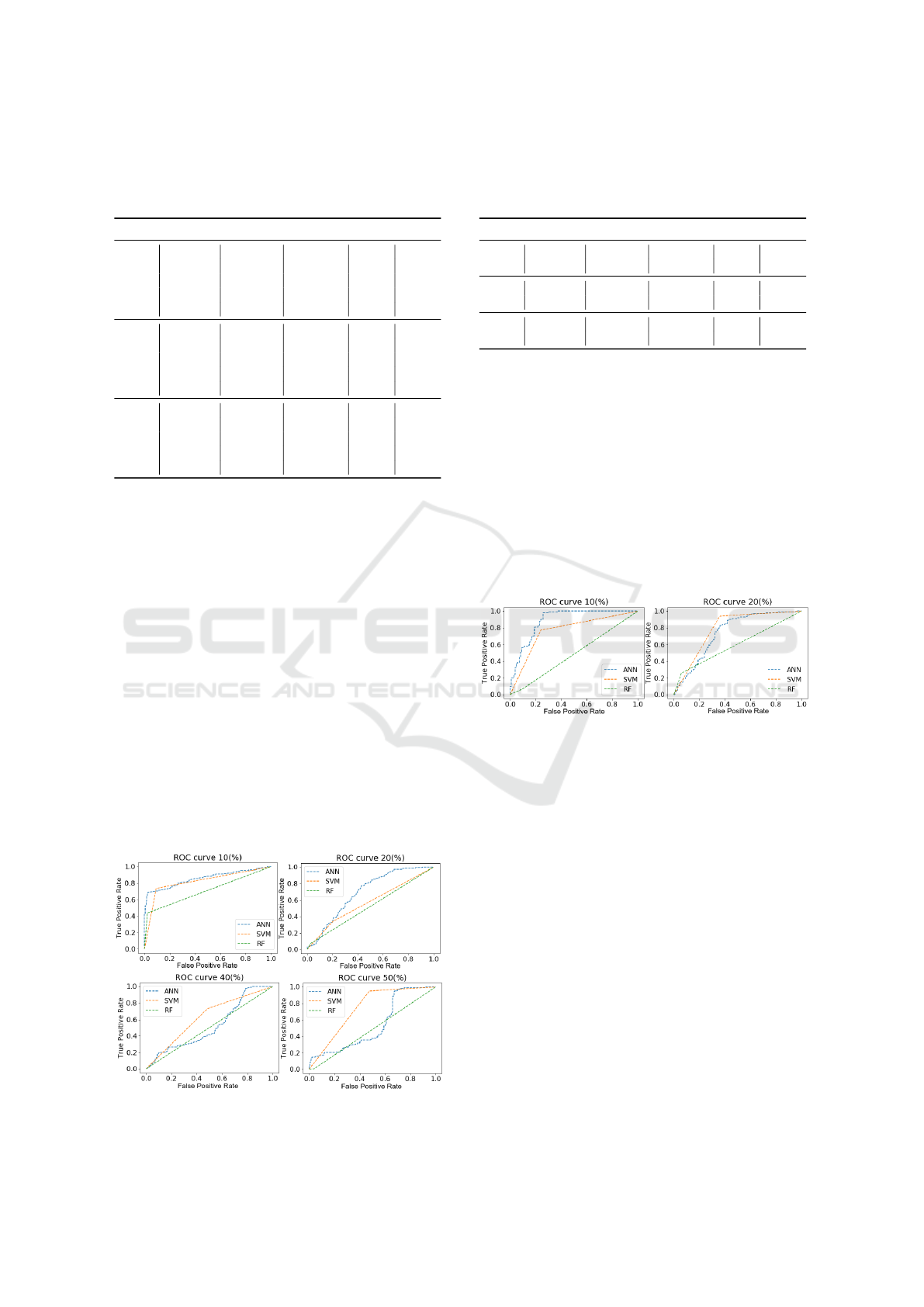
Table 4: Results ML algorithms for substitution with all

features H/ACA box: Area Under The Curve (AUC),

Matthews Correlation Coefﬁcient (MCC), Recall (R) and

Precision (P).

ML Datasets AUC(%) MCC(%) R(%) P(%)

10(%) 74.20 50.03 71.08 75.83

20(%) 63.22 30.02 40.41 74.35

ANN 30(%) 64.66 32.98 51.53 69.92

40(%) 58.14 22.71 21.41 80.70

50(%) 59.08 23.15 29.41 72.29

10(%) 67.76 36.37 55.12 73.76

20(%) 66.20 33.29 54.9 70.99

SVM 30(%) 64.33 29.23 65.63 63.99

40(%) 61.34 24.17 70.53 59.60

50(%) 61.36 22.78 54.85 63.06

10(%) 62.03 28.86 27.51 88.75

20(%) 52.75 2.38 17.43 59.37

RF 30(%) 60.64 21.59 29.47 78.29

40(%) 52.42 7.19 6.81 77.64

50(%) 50.57 2.92 4.52 57.24

where biological characteristics are not known, we

also tested the ML algorithms with a reduced number

of features, in this case zscore, AC, GU, GC, LloopSC,

RloopSC, LloopYC, and RloopYC. The three classi-

ﬁers performed poorly on all datasets, with an AUC

below 65%.

Insertion. Table 5 shows the results of the three ML

algorithms for the insertion experiment. In this ex-

periment, the mutation tree only generated sequences

recognized as H/ACA box by snoReport 2.0 up to

20% mutation. We could observe that the length of

the snoRNA sequence is an important feature for its

identiﬁcation.

The three classiﬁers presented a performance with

10% mutation higher than with 20% mutation. How-

ever, all metrics are close to or below 70%, see ﬁg 7.

Only ANN and SVM showed AUC and Recall greater

than 70% with 10% mutation. The results of the

three classiﬁers with 20 % mutation corresponding

Figure 6: ROC curves of the datasets with 10%, 20%, 40%

and 50% of mutation, for substitution, with all features.

Table 5: Results ML algorithms for insertion with all

features H/ACA box: Area Under The Curve (AUC),

Matthews Correlation Coefﬁcient (MCC), Recall (R) and

Precision (P).

ML Datasets AUC(%) MCC(%) R(%) P(%)

10(%) 71.92 47.90 59.31 79.3

ANN 20(%) 59.30 19.80 45.05 63.02

10(%) 74.76 51.45 80.4 72.31

SVM 20(%) 62.1 25.13 69.01 60.66

10(%) 59.79 22.83 28.91 75.65

RF 20(%) 51.21 1.81 28.32 52.29

to less than ideal performance. Again, we tested the

ML techniques with a reduced number of features:

zscore, AC, GU, GC, LloopSC, RloopSC, LloopYC,

and RloopYC. All three classiﬁers performed better

with 10% of mutations than with 20%, with the per-

formances decreasing further with the increasing of

number of mutations. For H/ACA box, the perfor-

mance of the AM classiﬁers were equivalent, using a

large number of known biological features as well as

a small number of them. For the insertion mutation,

the higher the percentage of mutation, the worse the

performance of the three classiﬁers.

Figure 7: ROC curve of the datasets 10% and 20%, for in-

sertion with all features.

4 CONCLUSION

In this article, we studied the performance of ML

methods to predict snoRNAs with the help of large

datasets built from artiﬁcially constructed mutation

trees. Even with limitations, we found that the ML

methods performed better than the most common con-

ventional homology search, Blast, which considers

only sequence similarity. As expected, the Blast re-

sults showed many false negative results for snoRNAs

with low sequence similarity to the query. For C/D

box, we observed that the ML methods consistently

performed better when provided with all known bi-

ologically relevant features. This was in particular

the case for the most diverged sequences. For the

substitution experiment, the SVM and ANN classi-

ﬁers achieved excellent performance for datasets with

10%, 20%, 30%, and 40% of mutations. A large drop

in performance was observed for 50% of mutations.

BIOINFORMATICS 2021 - 12th International Conference on Bioinformatics Models, Methods and Algorithms

182

For H/ACA box, the performance of the ML classi-

ﬁers, both using the full set of known biological char-

acteristics and a reduced number of features, showed

equivalent prediction performance. In the experiment

with the insertion mutation, performance decreased

with increasing mutation levels for all the three ML

classiﬁers.

In summary, our results show that ML methods

can be competitive with traditional homology search

methods, provided sufﬁciently large sets of indepen-

dent instances for test and training sets. This require-

ment, however, is prohibitive for most practical appli-

cations. We therefore suggest that the careful produc-

tion of artiﬁcial data is a promising approach that can

be pursued in practice, at least for families of ncRNAs

for which an adequate diverse set of representatives is

available. Our data also indicate that the knowledge

of a sufﬁciently large set of biologically relevant fea-

tures is important for the performance of ML-based

homology search.

Clearly, the present study is only a ﬁrst step.

It remains open whether the ML methods can also

compete with more sophisticated methods of homol-

ogy search such as Hidden Markov Models (HMMs)

(Eddy, 1996) or covariance models (CMs) (Nawrocki

and Eddy, 2013), which similar to ML models also

convey information of local and non-local correla-

tions, respectively.

REFERENCES

Achawanantakun, R., Chen, J., Sun, Y., and Zhang, Y.

(2015). LncRNA-ID: Long non-coding RNA IDentiﬁ-

cation using balanced random forests. Bioinformatics,

31(24):3897–3905.

Altschul, S. F., Gish, W., Miller, W., Myers, E. W., and

Lipman, D. J. (1990). Basic local alignment search

tool. J. Mol. Biol., 215(3):403–410.

Barber, D. (2012). Bayesian Reasoning and Machine

Learning. Cambridge University Press, Cambridge,

UK.

Bartschat, S., Kehr, S., Tafer, H., Stadler, P. F., and Hertel,

J. (2014). snoStrip: a snoRNA annotation pipeline.

Bioinformatics, 30(1):115–116.

Bratkovi

c, T., Bo

c, J., and Rogelj, B. (2020). Functional

diversity of small nucleolar RNAs. Nucleic Acids Re-

search, 48(4):1627–1651.

Breiman, L. (2001). Random forests. Machine Learning,

45:5–32.

de Araujo Oliveira, J. V., Costa, F., Backofen, R., Stadler,

P. F., Machado Telles Walter, M. E., and Hertel, J.

(2016). SnoReport 2.0: new features and a reﬁned

Support Vector Machine to improve snoRNA identiﬁ-

cation. BMC Bioinformatics, 17 Suppl. 18:464.

Eddy, S. R. (1996). Hidden Markov models. Current Op.

Struct. Biol., 6:361–365.

Falaleeva, M. and Stamm, S. (2013). Processing of snoR-

NAs as a new source of regulatory non-coding RNAs:

snoRNA fragments form a new class of functional

RNAs. BioEssays, 35(1):46–54.

Georgakilas, G. K., Grioni, A., Liakos, K. G., Chalupova,

E., Plessas, F. C., and Alexiou, P. (2020). Multi-

branch Convolutional Neural Network for Identiﬁca-

tion of Small Non-coding RNA genomic loci. Scien-

tiﬁc Reports, 10(1):9486.

Goldschmidt, R. and Passos, E. (2005). Data mining: a

Practical guide. Gulf Professional Publishing.

Gruber, A. R., Findeiß, S., Washietl, S., Hofacker, I. L., and

Stadler, P. F. (2010). RNAz 2.0: improved noncoding

RNA detection. Pac. Symp. Biocomput., 15:69–79.

Gulli, A. and Pal, S. (2017). Deep Learning with Keras.

Packt Publishing Ltd, Birmingham, UK.

Haykin, S. (1999). Neural Networks: A Comprehensive

Foundation. Prentice-Hall, Englewood Cliffs.

Lorenz, R., Bernhart, S. H., H

oner zu Siederdissen, C.,

Tafer, H., Flamm, C., Stadler, P. F., and Hofacker, I. L.

(2011). ViennaRNA Package 2.0. Alg. Mol. Biol.,

6:26.

Nawrocki, E. P. and Eddy, S. R. (2013). Infernal 1.1: 100-

fold faster RNA homology searches. Bioinformatics,

29(22):2933–2935.

Pedregosa, F., Varoquaux, G., Gramfort, A., Michel, V.,

Thirion, B., Grisel, O., Blondel, M., Prettenhofer, P.,

Weiss, R., Dubourg, V., Vanderplas, J. T., Passos, A.,

Cournapeau, D., Brucher, M., Perrot, M., and Duch-

esnay,

E. (2011). Scikit-learn: Machine learning in

python. J. Machine Learning Res., 12:2825–2830.

Rastogi, A. and Gupta, D. (2014). GFF-Ex: a genome fea-

ture extraction package. BMC research notes, 7:315.

Russell, S. and Norvig, P. (2010). Artiﬁcial Intelligence: A

Modern Approach. Prentice-Hall, Englewood Cliffs,

3nd edition.

Satoh, N. (2003). The ascidian tadpole larva: compara-

tive molecular development and genomics. Nature Re-

views Genetics, 4(4):285–295.

Waldl, M., Thiel, B., Ochsenreiter, R., Holzenleiter, A.,

de Araujo Oliveira, J. V., Walter, M. E. M. T., Wolﬁn-

ger, M. T., and Stadler, P. F. (2018). TERribly difﬁcult:

Searching for telomerase RNAs in Saccharomycetes.

Genes, 9:372.

Zhang, Y., Huang, H., Zhang, D., Qiu, J., Yang, J., Wang,

K., Zhu, L., Fan, J., and Yang, J. (2017). A Review on

Recent Computational Methods for Predicting Non-

coding RNAs. BioMed Res. Intl., 2017:1–14.

Zhang, Y. and Rajapakse, J. C. (2009). Machine Learning

in Bioinformatics. John Wiley & Sons, Hoboken, NJ.

Machine Learning Studies of Non-coding RNAs based on Artiﬁcially Constructed Training Data

183