
Bet-based Evolutionary Algorithms:
Self-improving Dynamics in Offspring Generation
Simon Reichhuber
a
and Sven Tomforde
b
Intelligent Systems, University of Kiel, Hermann-Rodewald-Str. 3, Kiel, Germany
Keywords:
Evolutionary Computation, Genetic Algorithms, Optimisation, Fitness Landscapes, Diversity, Bet-based
Approach.
Abstract:
Evolutionary Algorithms (EA) are a well-studied field in nature-inspired optimisation. Their success over the
last decades has led to a large number of extensions, which are particularly suitable for certain characteristics
of specific problems. Alternatively, variants of the basic approach have been proposed, for example to increase
efficiency. In this paper, we focus on the latter: We propose to enrich the evolutionary problem with a self-
controlling betting strategy to optimise the evolution of individuals over successive generations. For this
purpose, each individual is given a betting parameter to be co-optimised, which allows him to improve his
chances of “survival” by betting. We analyse the behaviour of our approach compared to standard procedures
by using a reference set of complex functional problems.
1 INTRODUCTION
The field of Evolutionary Computing (EC) comprises
four basic directions: evolutionary programming (EP)
(Fogel et al., 1966), evolution strategies (ES) (Schwe-
fel, 1965; Rechenberg, 1978), genetic algorithms
(GA) (Holland, 1975), and genetic programming
(GP) (Koza and Koza, 1992). Based on this original
work, an integrated field of research has developed.
The underlying processes have been successively de-
veloped and solutions for a wide range of prob-
lems have been proposed. Alternatively, novel ap-
proaches and improvements in the algorithmic logic
were presented, which aim at a higher robustness (see,
e.g., (Eiben and Smit, 2011)), the handling of noise
and uncertainty (see, e.g., (Jin and Branke, 2005)),
the consideration of security concerns (see, e.g., (Pro-
thmann et al., 2009)) or the consideration of different
objective functions (see, e.g., (Zelinka, 2015)).
In this paper, we look at an alternative approach to
generating the next population. Combined with an eli-
tist strategy and based on the objective of maintaining
diversity, especially in dynamic problems, we extend
the basic procedure by a possibility for each individ-
ual to temporarily increase their selection despite their
currently limited fitness. The individuals are given an
a
https://orcid.org/0000-0001-8951-8962
b
https://orcid.org/0000-0002-5825-8915
additional parameter with which they can invest a so-
called ’bet’ with regard to their fitness. This parame-
ter should then also be the focus of the optimisation.
Additionally, we suggest an approach in which an-
other external population is evolved to optimally bet
on another population.
The remainder of this paper is organised as fol-
lows: Section 2 introduces the basic terms and foun-
dations of this paper. Since the field of EAs is very
broad and heterogeneous, we determine a reference
approach in Section 3. Afterwards, Section 4 intro-
duces our novel bet-based approach. Section 5 anal-
ysis the behaviour of the approach in comparison to
other approaches (especially the reference) by consid-
ering optimisation problems defined by a set of stan-
dard mathematical functions. Finally, Section 6 sum-
marises the paper and gives an outlook to future work.
2 BACKGROUND
Holland et al. invented an optimisation technique that
is nowadays known as the canonical version of Ge-
netic Algorithms (GA) in 1975. Inspired by the nat-
ural evolutionary process, this stochastic optimisation
technique uses selection, recombination, and muta-
tion to evolve a set of binary solution strings denoted
as the population. The members of the population
are called chromosomes and are represented as vec-
1192
Reichhuber, S. and Tomforde, S.
Bet-based Evolutionary Algorithms: Self-improving Dynamics in Offspring Generation.
DOI: 10.5220/0010345611921199
In Proceedings of the 13th International Conference on Agents and Artificial Intelligence (ICAART 2021) - Volume 2, pages 1192-1199
ISBN: 978-989-758-484-8
Copyright
c
2021 by SCITEPRESS – Science and Technology Publications, Lda. All rights reserved

tors, where each entry is called a gene. Algorithm 1
represents one GA run: First, the initial population
is randomly drawn from a uniform random distribu-
tion. Second, the fitness value of each chromosome in
the population is calculated and based on this fitness
value a subset of the population, namely the parents,
are separated from the rest. These parents will now be
recombinated and a new offspring generation is born.
Finally, the parents and the new offspring generation
are mutated with a small probability and both of them
represent the next generation. After a certain genera-
tion is reached or the fitness value of the best chromo-
some exceeds a predefined threshold, the best found
solution is returned.
Algorithm 1: The canonical GA algorithm.
P = Initialization();
t = 0;
while error(t) > τ do
Fitness = CalculateFitness(P);
Parents = Selection(P);
Offspring = Recombination(Parents);
P = Mutation(Offspring);
t ← t + 1;
end
Result: x
ga
(t), y
ga
(t), t
Later, researchers expanded the canonical version
to also deal with real-valued problems (Wright,
1991; Goldberg, 1991; Eshelman and Schaffer, 1993;
Blanco et al., 2001). One key question was how to
find an adaptation mechanism which is able to adjust
the parameters of the EA during run. Here, the main
focus was on the step-size representing the differ-
ence of a chromosome before and after a single muta-
tion (Price, 1996; Azad and Hasanc¸ebi, 2014). Other
authors refined one of the genetic operations, such as
a uniform crossover (Syswerda, 1989) or arithmetic
recombination types (Michalewicz, 2013). All these
findings are improved optimisation algorithms, which
try to maximise or minimise an objective function.
For the purpose of generality, we focus on a wide va-
riety of not necessarily continuous functions and in-
troduce the optimisation problem formally. The op-
timisation problem is formulated as a constraint min-
imisation problem of functions f : R
d
→ R:
min
x
x
x∈R
d
f (x
x
x)
where a ≤ x
i
≤ b for i = 1,.. .,d
For each of the test functions f
1
− f
23
found in (Yao
and Liu, 1996; Yao and Liu, 1996; Cakar et al., 2011),
we call the function value of the global minimum
y
∗
= min
x
x
x∈[a,b]
d
f (x
x
x) and measure the error of the min-
imum value found by the genetic algorithm after the
t −th generation.
error(t) = |y
∗
−y
ga
(t)|
Additionally, we observe the number of generations
t
ga
required to reduce the error up to a tolerance τ
t
ga
= min
t∈N
where error(t) ≤ τ
3 REFERENCE EXTENSIONS IN
EVOLUTIONARY
ALGORITHMS
Since the field of EAs is very broad and heteroge-
neous, we first determine a reference approach. This
should then serve a basis for comparisons for the bet-
based approach developed in the next section. Before
we present the reference, we introduce basic EAs op-
erators that we used as the baseline for comparison
but also as starting point of the bet-based EAs. For
comparison of our bet-based genetic algorithms, we
introduce a baseline, based on the canonical genetic
algorithm. Therefore, we describe the steps of the EA.
Initialise Population. The population P is uni-
formly chosen from the hypercube [a, b]
d
. N chro-
mosomes x
x
x
i
∈ P are drawn.
Fitness Function. Since all the functions are min-
imisation problems including negative output values,
we define our fitness function as follows:
F(x
x
x
i
) = −( f (x
x
x) −y
min
(P)),
where y
min
(P) = min
x
x
x∈P
f (x
x
x) is the worst fitness
value.
Selection. The parent population is found with re-
spect to the fitness values of the chromosomes. The
na
¨
ıve selection strategy that takes the top k chromo-
somes into account leads to a poor diversity of the
next generations. Stochastic selection strategies solve
the latter. We used the two selection strategies re-
mainder stochastic sampling and universal sampling.
The remainder stochastic sampling is based on (Hol-
land, 1975; Goldberg, 1991; Blanco et al., 2001) on
the relative fitness.
F
rel
(x
x
x
i
) =
F(x
x
x
i
)
F
,
where F =
1
N
∑
N
i=1
F(x
x
x
i
) is the mean fitness value.
Here, chromosomes x
x
x
i
i
i
∈ P with a relative fitness
Bet-based Evolutionary Algorithms: Self-improving Dynamics in Offspring Generation
1193

larger or equal than 1, i.e. F
rel
≥ 1 are copied
bF
rel
(x
x
x
i
)ctimes to the parent population and the resid-
ual F
rel
(x
x
x
i
)−bF
rel
(x
x
x
i
)c and all other fitness values be-
low 1 represent the probability of copying the corre-
sponding chromosome to the parent selection. Analo-
gously, universal sampling is a selection strategy with
replacement where chromosomes are selected accord-
ing to the probability:
p(x
x
x) =
F(x
x
x
i
)
∑
N
i=1
F(x
x
x
i
)
.
For both strategies, there are drawn N
P
parents.
Offspring and Recombination. Recombination is
done by applying a crossover of a pair of parents. This
procedure is repeated until N −N
P
children has been
created. As we want to focus on a diversity of the off-
spring generation, we choose the uniform crossover
(Syswerda, 1989; De Jong and Spears, 1990) in all of
our experiments. Specifically, for child 1 each gene
is either taken from parent 1 or parent 2 with equal
probability and the other child is given as the inverse
of child 1 (see Algorithm 2).
Algorithm 2: Recombination procedure with uni-
form crossover.
Offspring =
/
0;
while |Offspring| < N −N
P
do
Parent
1
,Parent
2
=
random nonequal tuple(Parents);
if p
r
≤ uni f orm([0,1]) then
Offspring
1
,Offspring
2
=
uni f orm crossover(Parent
1
,Parent
2
);
Offspring ←
Offspring ∪{Offspring
1
,Offspring
2
}
end
end
Result: Offspring
Mutation. Finally, the next generation is obtained by
applying mutation on the parents and their offspring.
Three different mutation operations for real vectors
are discussed, random mutation (Blanco et al., 2001),
non-uniform mutation (Blanco et al., 2001), and one-
step mutation (Eiben and Smith, 2015). After ran-
domly choosing an amount of p
m
genes out of all N ∗d
possible genes, the genes x
x
x[i] are mutated by replac-
ing them with:
• Random mutation:
x
x
x[i]
0
drawn uniformly from the range [a,b].
• Non-uniform mutation:
x
x
x[i]
0
=
(
x
x
x[i] + ∆(t,b −x
x
x[i]) if γ = 0
x
x
x[i] + ∆(t,x
x
x[i] −a) if γ = 1
,
where γ is equally likely 0 or 1
and ∆(t, y) = y
1 −r
(1−t/g
max
)
κ
. κ controls the
degree of dependency on the number of iterations
g
max
, s.t. the higher κ the more likely the values of
∆, which lie in the range [0, y], are close to zero.
In Figure 1 the influence of this parameter is vi-
sualised for different values κ = 1,2,5 over 100
generations. One drawback of the non-uniform
mutation is that the number of iterations must be
known a priori. Therefore, this mutation can only
be applied for experiments with a fixed number of
generations.
• One-step mutation:
Based on the old gene x
x
x[i], x
x
x[i]
0
is
drawn uniformly from the interval
[max{a,x
x
x[i] −1},min{b,x
x
x[i] + 1}]
Elitism. Only, a small amount of the best chromo-
somes in the population, denoted as elites, are im-
mune to the mutation operation and are added directly
to the next generation. Therefore, the parameter r
elite
defines the fraction of elites in the population.
4 NOVEL APPROACHES TO
BET-BASED EVOLUTIONARY
ALGORITHMS
The following idea led us to the approach of bet-based
agents: Instead of directly solving the minimisation
problem, we convert it to a meta problem, which
we call bet-based problem, meaning instead of di-
rectly solving the problem and providing a minimum
x
∗
= min
x∈D
f (x) the algorithm learns to place an op-
timal bet on a near-to-optimal solution. In every it-
eration the algorithm approximate to the solution by
giving bets on x
x
x
1
,··· ,x
x
x
N
. By answering the question
who bets about what, we come up with two different
betting mechanisms:
• Self-betting EA (self BEA): Each chromosome of
the population bets egocentrically on its own fit-
ness increase. The bet parameters are encoded in
the genes of the individual.
• External-betting EA (external BEA): Another gen-
eration (bet population) bets on the population
that solves the minimisation (main population.)
In the remainder of this chapter, we present the two
approaches in detail.
ICAART 2021 - 13th International Conference on Agents and Artificial Intelligence
1194
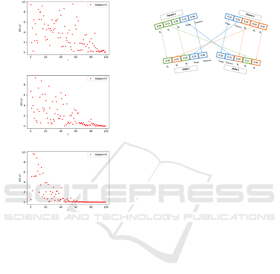
(a) κ = 1
(b) κ = 2
(c) κ = 5
Figure 1: Influence of the value κ on the mutation through
the iterations.
4.1 Self-betting EAs
We convert the canonical algorithm into a bet-based
EA by introducing new learning parameters that are
appended to the chromosomes. The first is used to
determine the bet amount c
wager
∈ [0,1] and the sec-
ond one is used to control the influence of the fitness
increase c
in f luence
∈ [0,1]. In case the function value
of the chromosome changes after a generation, to the
fitness value from Section 3 the bet outcome π(x
x
x) is
added, either in a positive (∆ f (x
x
x
i
) > 0) or negative
way (∆ f (x
x
x
i
) < 0), with the function difference after
one generation ∆ f (x
x
x
i
) = ∆ f (x
x
x
t
i
) = f (x
x
x
t+1
) − f (x
x
x
t
).
F
t+1
(x
x
x
i
) =F
t
(x
x
x
i
) +π(x
x
x
i
)
π(x
x
x
i
) =c
global
∗ f (x
x
x
i
) ∗sgn(∆ f (x
x
x
i
)) ∗(F
t
(x
x
x) ∗c
wager
)
∗(∆ f (x
x
x
i
) ∗c
in f luence
+ 1),
where c
global
is a constant that controls the bet influ-
ence, i.e. if c = 1 the maximal bet influence is as
high as the old function value. The betting mech-
anism leads to higher oscillation of fitness values.
Self BEA Crossover
Figure 2: Crossover in self-betting GA procedure.
Our assumption is that the betting mechanism pushes
the chance of survival for chromosomes that have re-
cently found new global maximum candidates.
Recombination. As we do not want to mix bet
genes with problem genes, we used a simple uniform
crossover for each of these parameter sets as visu-
alised in Figure 2.
Mutation. We use one of the three presented mu-
tation strategies but shrink the mutation range for the
bet parameters to the interval [0,1].
Elitism. Especially for elite chromosomes, the out-
come of the bet is always 0 since ∆ f (x
x
x) is 0. To pre-
vent weaker chromosomes from displacing the elite,
the elite status depends on the raw functional value.
All other mechanisms are exactly as discussed in
Section 3.
4.2 External-betting EAs
We call this approach external-betting EAs or simply
external BEAs. Beside the main population, we create
a second population, called the bet population, where
each individual is encoded as chromosomes consist-
ing of genes b
b
b
j
[i] ∈ [−1,1], j = 1,.. .,N
bet
, i =
1,... ,N
main
, where each gene represents a bet for a
specific chromosome of the main population. A posi-
tive value indicates that the bet chromosome bets on a
fitness increase of the chromosome of the main popu-
lation and a negative value indicates a bet on the de-
crease of the same (cf. Figure 4). As visualised in Fig-
ure 3, for the bet population the bet procedure starts
by placing bets and waiting for the outcome to recal-
culate the fitness value. The fitness values are updated
as follows:
F
bet
(b
b
b
j
) =
N
main
∑
i=1
b
b
b
j
[i] ∗∆ f (x
x
x
i
)
Bet-based Evolutionary Algorithms: Self-improving Dynamics in Offspring Generation
1195
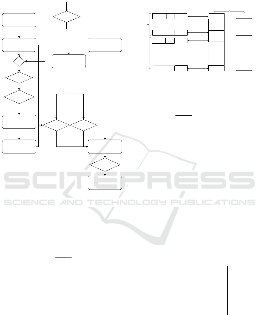
Main Population
Fitness
Bet Population
+
Next Main
Population
Winnings
Function Values
Bets
Function Values Fitness
GA Operations
Next Bet Population
GA Operations
Losses
Winnings
Figure 3: Bet procedure for external BEA.
On the other hand, the bets influences the fitness val-
ues of the next main population. More specific, only
won bets on fitness increase can influence the next
main population. The new fitness values are calcu-
lated as follows:
F
t+1
(x
x
x) =F
t
(x
x
x) + π(x
x
x)
π(x
x
x) =c
global
∗ f (x
x
x)
1
|P
bet,+
i
|
∑
b
b
b∈P
bet,+
i
b
b
b[i]
P
bet,+
i
:= {b
b
b ∈ P
bet
|b
b
b[i] > 0 ∧∆ f (x
x
x
i
) > 0},
where P
bet,+
i
is the set of a all chromosomes in the bet
population that have bet on an increase of the function
value of the chromosome x
x
x
i
of the main population
and have won.
Since the bet procedure is based on a 1-to-1 corre-
lation between the genes of a chromosomes in the bet
population and the chromosomes in the main popula-
tion, we have to reassign bet chromosome genes that
are obsolete after the offspring have displaced parts of
the main population. This is done by using a weighted
average of the bets of the parents. Based on the num-
ber of genes that had been chosen from parent 1 in the
Main Population
Bet Population
Population
…
…
parents
…
children
…
…
chromosomes
…
…
…
place bet
place bet
…
place bet
place bet
…
…
Figure 4: Betting in external BEA.
uniform crossover n
parent
1
and the number of genes of
parent 2 n
parent
2
the bet genes for the offspring are
calculated as follows:
b
b
b
j
[i] =
n
parent
2
d
∗ parent
1
(b
b
b
j
)[i]
+
n
parent
2
d
∗ parent
2
(b
b
b
j
)[i].
All other mechanisms are exactly as discussed in Sec-
tion 3, except the fact that we have to apply each ge-
netic operator double since we have two populations.
5 EXPERIMENTAL EVALUATION
For the experiments, we used the suggested numerical
problems in (Cakar et al., 2011) as defined in Table 3
and choose a 30 dimensions whenever the dimension
was adaptable. The first two dimensions of the func-
tions are visualised in Figure 5. To solve the hyper pa-
rameter optimisation of all discussed parameters, we
applied a grid search over all function by applying the
grid parameters in Table 1.
Table 1: Evaluated parameter grid and optimal parameters
found. Remainder stochastic sampling strategy is abbrevi-
ated as rss and universal stochastic sampling as us.
name range opt. param
selection [rsss,uss] rsss
mutation [rnd,non − uni.,1 −
step]
1 −step
parents ratio [0.25,0.5,0.75] 0.25
mutation rate [0,0.01,0.02,0.03] 0.01
elite rate [0,0.01,0.02, 0.03] 0.03
c
global
[0.1,0.3,0.5] 0.1
Here we observed the mean value over 5 runs, used a
fixed number of 100 generations and a population size
of 100. For the non-uniform mutation strategy, we
choose κ = 2 and the crossover type was a uniform
crossover. After ranking the parameter grid applied
over a single function, we took the sum of all ranked
ICAART 2021 - 13th International Conference on Agents and Artificial Intelligence
1196

Table 2: Comparison of the algorithms EA, self BEA, and
external BEA applied on 23 functions (see Table 3).
fun. err(GA) err(self BEA) err(ext. BEA)
f1 17.74 ±2.46 17.61 ±1.48 18.62 ±0.92
f2 37.12 ±4.01 40.1 ±13.67 35.12 ±6.57
f3 0.0 ±0.0 0.0 ±0.0 0.0 ±0.0
f4 12.18 ±5.1 28.61 ±8.17 21.31 ±4.36
f5 17e4 ±2.2e4 19e4 ±4.3e4 16e4 ±5.6e4
f6 19.0 ±1.9 18.2 ±2.93 19.0 ±2.19
f7 21.93 ±13.72 20.88 ±11.7 18.07 ±12.52
f8 2.6e3 ±1.6e3 2.9e3 ±0.3e3 2.7e3 ±1.5e3
f9 232.99 ±5.64 232.43 ±9.77 221.45 ±15.15
f10 4.34 ±0.16 13.67 ±7.36 4.12 ±0.14
f11 11.04 ±4.71 102.33 ±8.23 40.7 ±12.94
f12 5.31 ±1.0 6.25 ±1.11 4.94 ±1.21
f13 8.49 ±1.56 6.49 ±0.9 7.35 ±1.56
f14 3.15 ±3.0 3.9 ±5.11 1.97 ±2.42
f15 7e−4 ±3e−4 0.0 ±2e−4 0.0012 ±5e−4
f16 4e−4 ±4e−4 0.0 ±2e−4 4e−4 ±2e−4
f17 1e−4 ±1e−4 0.0 ±1e−4 1e−4 ±2e−4
f18 0.01 ±0.0071 0.0192 ±0.0098 0.0179 ±0.0097
f19 0.0018 ±0.0017 0.001 ±0.0017 0.0 ±0.0015
f20 0.21 ±0.03 0.25 ±0.04 0.17 ±0.06
f21 3.17 ±2.77 4.08 ±3.35 2.43 ±2.29
f22 1.01 ±0.29 1.99 ±2.87 0.75 ±0.22
f23 0.84 ±0.45 2.22 ±2.99 0.81 ±0.3
grids into consideration and found the best parame-
ter set as the minimum rank. For all the presented
algorithms, i.e. EA, self BEA, external BEA, these
optimal parameters were used for a longer test run,
in order to compare them. Over 10 runs, 500 gener-
ations and a population size of 100, we analysed the
mean of the remaining absolute error (cf. Table 2)
and the mean progress over the generations(cf. Fig-
ure 6). As result, for the functions the reference EAs
is better in 4 cases, the self BEAs in 6 cases, and the
external BEAs in 12 cases. The high standard devia-
tion of the algorithms self BEA and external BEA in
Figure 6 indicates a high variance in the population
but also shows that only in the long-term the two new
algorithms are able to beat the reference.
6 CONCLUSIONS
We gave a short recap of the history of EP and pre-
sented a variety of operations of EAs. In perspective
of these, we derived a reference EA for the compar-
ison of two new bet-based EAs, called self-betting
evolutionary algorithms (self BEAs) and external-
betting evolutionary algorithms (external BEAs).
These new bet-based algorithms are able to learn how
to successfully bet, either bet on themselves (self
BEAs) or on an external population (external BEAs).
We presented experiments on 23 high dimensional
test functions and showed that the new algorithms are
able to beat the reference in the majority of all anal-
Table 3: Numerical problems.
Function Dim d Ranges Minimum value
f
1
(x
x
x) =
∑
n
i=1
x
2
i
30 −100 −5.12 ≤x
i
≤ 5.12 f
1
(0
0
0) = 0
f
2
(x
x
x) =
∑
n
i=1
|x
i
|+
∏
n
i=1
x
i
30 −100 −10 ≤ x
i
≤ 10 f
2
(0
0
0) = 0
f
3
(x
x
x) =
∑
n
i=1
(
∑
i
j=1
x
i
)
2
30 −100 −100 ≤x
i
≤ 100 f
3
(0
0
0) = 0
f
4
(x
x
x) = max |x
i
|,0 ≤ i < n 30 −100 −100 ≤x
i
≤ 100 f
4
(0
0
0) = 0
f
5
(x
x
x) =
∑
n−1
i=1
(100 ·(x
i+1
−x
2
i
)
2
+ (x
i
−1)
2
) 30 −100 −30 ≤ x
i
≤ 30 f
5
(1
1
1) = 0
f
6
(x
x
x) =
∑
n
i=1
bx
i
+
1
2
c
2
30 −100 −1.28 ≤x
i
≤ 1.28
f
6
(p
p
p) = 0
−
1
2
≤ p
i
<
1
2
f
7
(x
x
x) = (
∑
n
i=1
(i +1) ·x
4
i
) +rand[0, 1[ 30 −100 −1.28 ≤x
i
< 1.28 f
7
(0
0
0) = 0
f
8
(x
x
x) =
∑
n
i=1
−x
i
·sin(
p
|x
i
|)
30 −100 −500 ≤x
i
≤ 500
f
8
(4
4
42
2
20
0
0.
.
.9
9
96
6
68
8
87
7
7) =
−418.9829 ∗d
f
9
(x
x
x) =
∑
n
i=1
(x
2
i
−10 ·cos (2πx
i
) +10) 30 −100 −5.12 ≤x
i
≤ 5.12 f
9
(0
0
0) = 0
f
10
(x
x
x) = −20 ·exp(−0.2
q
1
n
∑
n
i=1
x
2
i
)−
30 −100 −32 ≤ x
i
≤ 32 f
10
(0
0
0) = 0
exp(
1
n
∑
n
i=1
cos(2πx
i
)) +20 + e
f
11
(x
x
x) =
1
4000
∑
n
i=1
x
2
i
+
∏
n
i=1
cos
x
i
√
i+1
30 −100 −600 ≤x
i
≤ 600 f
11
(0
0
0) = 0
f
12
(x
x
x) =
π
n
10 ·(sin (πy
1
))
2
30 −100 −50 ≤ x
i
≤ 50 f
12
(−
−
−1
1
1) = 0
+
∑
n−1
i=1
(y
i
−1)
2
·
1 + 10
˙
(sin (πy
i+1
))
2
+(y
n
−1)
2
+
∑
n
i=1
u(x
i
,5, 100,4)
f
13
(x
x
x) = 0.1
(sin(3πx
1
))
2
30 −100 −50 ≤ x
i
≤ 50 f
13
(1
1
1) = 0
∑
n−1
i=1
(x
i
−1)
2
·
sin(3πx
i+1
)
2
+ (x
n
−1)
·
1 + (sin (2πx
n
))
2
+
∑
n
i=1
u(x
i
,5, 100,4)
f
14
(x
x
x) =
1
500
+
∑
25
j=1
j +
∑
2
i=1
(x
i
−a
i j
)
6
−1
−1
2 −65.54 ≤x
i
≤ 65.54 f
14
(−
−
−3
3
32
2
2) = 0.9980
f
15
(x
x
x) =
∑
11
i=1
a
i
−
x
1
(b
2
i
+b
i
x
1
)
b
2
i
+b
i
x
2
+x
3
2
4 −5 ≤x
i
≤ 5
f
15
(.19,.19, .12,.14)
= 3.42e−4
f
16
(x
x
x) = 4x
2
0
−2.1x
4
0
+
1
3
x
6
0
+ x
0
x
1
−4x
2
1
+ 4x
4
1
2 −5 ≤x
i
≤ 5
f
16
(0.09,−0.71)
= −1.032
f
17
(x
x
x) = (x
1
−
5.1
4π
2
x
2
0
+
5
π
x
0
−6)
2
2 −5 ≤x
i
≤ 15
f
17
(−3.14,12.26)
+10 ·(1 −
1
8π
) ·cos (x
0
) +10 = 0.398
f
18
(x
x
x) =
1 + (x
0
+ x
1
+ 1)
2
·(19 −14x
0
+ 3x
2
0
−14x
1
2 −2 ≤x
i
≤ 2 f
18
(0,−1) = 3
+6x
0
x
1
+ 3x
2
1
)
·
30 + (2x
0
−3x
1
)
2
·(18 −32x
0
+ 12x
2
0
+ 48x
1
−36x
0
x
1
+ 27x
2
1
)
f
19
= −
∑
4
i=1
c
i
exp
−
∑
3
j=1
a
i j
(x
j
−p
i j
)
2
4 0 ≤x
i
≤ 1
f
19
(.114,.556, .852)
= −3.86
f
20
= −
∑
4
i=1
c
i
exp
−
∑
6
j=1
a
i j
(x
j
−p
i j
)
2
4 0 ≤x
i
≤ 1
f
20
(.201,.150, .477,
.275,.311, .657)
= −3.32
f
21
(x
x
x) = −
∑
5
i=1
(x −a
i
)
T
(x −a
i
) +c
i
−1
4 0 ≤ x
i
≤ 10 f
21
(4
4
4) = −10.15
f
22
(x
x
x) = −
∑
7
i=1
(x −a
i
)
T
(x −a
i
) +c
i
−1
4 0 ≤ x
i
≤ 10 f
22
(4
4
4) = −10.40
f
23
(x
x
x) = −
∑
10
i=1
(x −a
i
)
T
(x −a
i
) +c
i
−1
4 0 ≤ x
i
≤ 10 f
23
(4
4
4) = −10.54
Functions for f
12
, f
13
: Vectors a, b for f
15
:
u(x,u, v,w) =
v(x −u)
w
if x > u
0 if x < −u
v(−x −u)
w
if −u ≤ x ≤ u
a = (.1957,.1947, .1735,.1600, .0844,
.0627,.0456, .0342,.0323, .0235,.0246)
y
i
= 1 +
1
4
(x
i
+ 1) b
−1
i
= (0.25,0.5, 1,2, 4,6, 8,10, 12,14, 16)
2 ×25 matrix a for f
14
:
(a
i j
) =
−32 −16 0 16 32 −32 . .. 0 16 32
−32 −32 −32 −32 −32 −16 . .. 32 32 32
4 ×3 matrices a, p and vector c for f
19
(a
i j
) =
3 10 30
.1 10 35
3 10 30
.1 10 35
(p
i j
) =
.3689 .1170 .2673
.4699 .4387 .7470
.1091 .8732 .5547
.038150 .5743 .8828
c = (1,1.2, 3,3.2)
4 ×6 matrices a, p and vector c for f
20
:
(a
i j
) =
10 3 17 3.5 1.7 8
.05 10 17 .1 8 14
3 3.5 1.7 10 17 8
17 8 .05 10 .1 14
(p
i j
) =
.1312 .1696 .5569 .0124 .8283 .5886
.2329 .4135 .8307 .3736 .1004 .9991
.2348 .1415 .3522 .2883 .3047 .6650
.4047 .8828 .8732 .5743 .1091 .0381
c = (1,1.2, 3,3.2)
10 ×4 matrix a and vector c for f
21
, f
22
, f
23
(a
i j
) =
4 4 4 4
1 1 1 1
8 8 8 8
6 6 6 6
3 7 3 7
2 9 2 9
5 5 3 3
8 1 8 1
6 2 6 2
7 3.6 7 3.6
c = (.1,.2, .2,.4, .4,.6, .3,.7, .5,.5)
ysed test functions. As discussed in (Ghoreishi et al.,
2017), the stopping criterion plays an important role
for the practical applicability of EAs. Since our ex-
periments provide evidence of an advantage of bet-
based EAs over canonical EAs after a fixed number
of function evaluations, an analysis of suitable stop
criteria for bet-based EAs should be investigated in
further research. We assume that for example choos-
ing the k -iteration stop criterion, where the algorithm
stops after a period of k iterations without improve-
ment, the bet-based EAs may use this duration more
efficiently. That is, the dynamic of bets pushes weak
chromosomes on their way to the global optimum and
let them dominate over chromosomes that are trapped
in local optima. Additionally to the latter, for further
research we want to extend the test procedure to learn
how the designed algorithms can be refined. Also,
Bet-based Evolutionary Algorithms: Self-improving Dynamics in Offspring Generation
1197
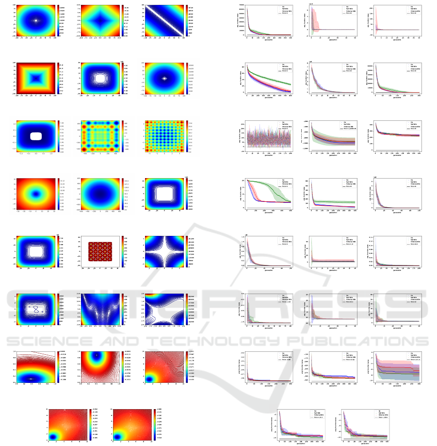
(a) f
1
(b) f
2
(c) f
3
(d) f
4
(e) f
5
(f) f
6
(g) f
7
(h) f
8
(i) f
9
(j) f
10
(k) f
11
(l) f
12
(m) f
13
(n) f
14
(o) f
15
(p) f
16
(q) f
17
(r) f
18
(s) f
19
(t) f
20
(u) f
21
(v) f
22
(w) f
23
Figure 5: Functions specified in 3 found in (Yao et al.,
1999). Only the first two dimensions are visualised.
we want to adapt the betting mechanism to machine
learning models that can be evolved.
REFERENCES
Azad, S. K. and Hasanc¸ebi, O. (2014). An elitist self-
adaptive step-size search for structural design opti-
mization. Applied Soft Computing, 19:226 – 235.
Blanco, A., Delgado, M., and Pegalajar, M. C. (2001).
(a) f
1
(b) f
2
(c) f
3
(d) f
4
(e) f
5
(f) f
6
(g) f
7
(h) f
8
(i) f
9
(j) f
10
(k) f
11
(l) f
12
(m) f
13
(n) f
14
(o) f
15
(p) f
16
(q) f
17
(r) f
18
(s) f
19
(t) f
20
(u) f
21
(v) f
22
(w) f
23
Figure 6: Comparison of the algorithms EA, self BEA, and
external BEA applied on 23 functions (see Table 3).
A real-coded genetic algorithm for training recurrent
neural networks. Neural networks, 14(1):93–105.
Cakar, E., Tomforde, S., and M
¨
uller-Schloer, C. (2011). A
role-based imitation algorithm for the optimisation in
dynamic fitness landscapes. In 2011 IEEE Symposium
on Swarm Intelligence, pages 1–8.
De Jong, K. A. and Spears, W. M. (1990). An analysis of
the interacting roles of population size and crossover
in genetic algorithms. In International Conference on
Parallel Problem Solving from Nature, pages 38–47.
Springer.
ICAART 2021 - 13th International Conference on Agents and Artificial Intelligence
1198

Eiben, A. E. and Smit, S. K. (2011). Parameter tuning for
configuring and analyzing evolutionary algorithms.
Swarm and Evolutionary Computation, 1(1):19–31.
Eiben, A. E. and Smith, J. E. (2015). Introduction to evolu-
tionary computing. Springer.
Eshelman, L. J. and Schaffer, J. D. (1993). Real-coded ge-
netic algorithms and interval-schemata. In Founda-
tions of genetic algorithms, volume 2, pages 187–202.
Elsevier.
Fogel, L. J., Owens, A. J., and Walsh, M. J. (1966). Artifi-
cial intelligence through simulated evolution.
Ghoreishi, S. N., Clausen, A., and Joergensen, B. N. (2017).
Termination criteria in evolutionary algorithms: A
survey. In Proceedings of the 9th International Joint
Conference on Computational Intelligence - IJCCI,,
pages 373–384. INSTICC, SciTePress.
Goldberg, D. (1991). Real-coded genetic algorithms, virtual
alphabets, and blocking. Complex Syst., 5.
Holland, J. (1975). Adaptation in natural and artificial sys-
tems, univ. of mich. press. Ann Arbor.
Jin, Y. and Branke, J. (2005). Evolutionary optimization in
uncertain environments-a survey. IEEE Transactions
on evolutionary computation, 9(3):303–317.
Koza, J. R. and Koza, J. R. (1992). Genetic programming:
on the programming of computers by means of natural
selection, volume 1. MIT press.
Michalewicz, Z. (2013). Genetic algorithms+ data struc-
tures= evolution programs. Springer Science & Busi-
ness Media.
Price, K. V. (1996). Differential evolution: a fast and simple
numerical optimizer. In Proceedings of North Ameri-
can Fuzzy Information Processing, pages 524–527.
Prothmann, H., Branke, J., Schmeck, H., Tomforde, S.,
Rochner, F., H
¨
ahner, J., and M
¨
uller-Schloer, C.
(2009). Organic traffic light control for urban road net-
works. Int. J. Auton. Adapt. Commun. Syst., 2(3):203–
225.
Rechenberg, I. (1978). Evolutionsstrategien. In Simula-
tionsmethoden in der Medizin und Biologie, pages 83–
114. Springer.
Schwefel, H.-P. (1965). Kybernetische evolution als strate-
gie der experimentellen forschung in der stromung-
stechnik. Diploma thesis, Technical Univ. of Berlin.
Syswerda, G. (1989). Uniform crossover in genetic algo-
rithms. In Proceedings of the 3rd international con-
ference on genetic algorithms, pages 2–9.
Wright, A. H. (1991). Genetic algorithms for real parameter
optimization. In Foundations of genetic algorithms,
volume 1, pages 205–218. Elsevier.
Yao, X. and Liu, Y. (1996). Fast evolutionary programming.
Evolutionary programming, 3:451–460.
Yao, X., Liu, Y., and Lin, G. (1999). Evolutionary program-
ming made faster. IEEE Transactions on Evolutionary
computation, 3(2):82–102.
Zelinka, I. (2015). A survey on evolutionary algorithms
dynamics and its complexity–mutual relations, past,
present and future. Swarm and Evolutionary Compu-
tation, 25:2–14.
Bet-based Evolutionary Algorithms: Self-improving Dynamics in Offspring Generation
1199
