
Path Planning for Autonomous Vehicles with Dynamic Lane Mapping
and Obstacle Avoidance
Ahmed El Mahdawy and Amr El Mougy
Department of Computer Science and Engineering, German University in Cairo, Cairo, Egypt
Keywords:
Autonomous Vehicles, Path Planning, Obstacle Avoidance.
Abstract:
Path planning is at the core of autonomous driving capabilities, and obstacle avoidance is a fundamental part
of autonomous vehicles as it has a great effect on passenger safety. One of the challenges of path planning
is building an accurate map that responds to changes in the drivable area. In this paper, we present a novel
path planning model with static and moving obstacle avoidance capabilities, LiDAR-based localization, and
dynamic lane mapping according to road width. We describe our cost-based map building approach and show
the vehicle trajectory model. Then, we evaluate our model by performing a simulation test as well as a real
life demo, in which the proposed model proves to be effective at maneuvering around static road obstacles, as
well as avoiding collisions with moving obstacles such as in pedestrian crossing scenarios.
1 INTRODUCTION
Road traffic injuries kill approximately 1.35 million
people each year (WHO, 2020). Among the pri-
mary risk factors for road traffic deaths are speed-
ing, distracted driving and driving under the influ-
ence, all preventable human errors (WHO, 2020). Au-
tonomous driving features have the power to alert the
driver of surrounding dangers and potentially fatal er-
rors. Fully autonomous driving systems have to be
aware of the vehicle’s surroundings with high accu-
racy, and need to be able to plan ahead the motion of
the vehicle in a way that does not impose any danger
on surrounding pedestrians or traffic, while maintain-
ing some level of driving comfort inside the vehicle
by reducing sudden acceleration or changes of direc-
tion of the vehicle.
Path planning is the means by which autonomous
vehicles plan ahead their movements and navigate
through the environment. There are multiple chal-
lenges in planning an autonomous vehicle’s path
through a dynamic environment:
1. Building an offline coordinate-based map that will
provide a basis for the vehicle’s real-world posi-
tion and its planned trajectory.
2. Localizing the vehicle’s current position on the
map, and planning a short-term path through these
points. There can be multiple candidate points for
the vehicle’s next step. The best candidate must
be decided based on the positions of the obstacles
(e.g. traffic and pedestrians) detected by the vehi-
cle’s sensing modules.
3. Finding the best heading and acceleration for the
vehicle to ensure a safe path possibly also taking
comfortability into account (favouring smoother
paths with less sudden acceleration).
Grid-based approaches are commonly used for the of-
fline map, representing the drivable environment as a
set of grid cells (called waypoints) with fixed posi-
tions.
Acquiring accurate information about the vehi-
cle’s position is essential for path generation. GPS-
based approaches may not provide the needed accu-
racy for autonomous navigation. Another approach
is to use a pre-generated point cloud map stored on
the vehicle. A point cloud map is a set of 3D points
mapping the environment, usually recorded from live
LiDAR data.
In the path finding step, given that a map of the
environment exists and we know the current position
of the vehicle on the map, we are interested in gener-
ating a plan of the ideal path for vehicle over the next
few seconds. This plan should be in the same domain
as the environment map (meaning that we are not con-
cerned with the vehicle’s exact trajectory yet, only its
next positions on the map).
A cost function provides a way to numerically rep-
resent the likeliness that any given selection in the ve-
El Mahdawy, A. and El Mougy, A.
Path Planning for Autonomous Vehicles with Dynamic Lane Mapping and Obstacle Avoidance.
DOI: 10.5220/0010342704310438
In Proceedings of the 13th International Conference on Agents and Artificial Intelligence (ICAART 2021) - Volume 1, pages 431-438
ISBN: 978-989-758-484-8
Copyright
c
2021 by SCITEPRESS – Science and Technology Publications, Lda. All rights reserved
431

hicle’s path is the most ideal one. In the case of grid-
based maps they can be used to assign a cost value
to each node in the grid. A shortest path algorithm
can then take into account these costs in order to find
a path of least cumulative cost. Cost functions must
take into account the chance of collision that is intro-
duced by taking a given path. A cost function should
never favor a path that puts the vehicle into a collision
trajectory. Cost functions may also consider the com-
fortability of a given path based on factors such as the
frequency of lane switches (Boroujeni et al., 2017), or
the acceleration or jerk in the generated path (Elban-
hawi et al., 2015).
The vehicle trajectory step involves transforming
the motion plan from the environment map domain
into real-world physical coordinates, and creating a
trajectory plan that steers the vehicle along the nodes
of the generated path. In some grid-based approaches,
cubic spline interpolation is used to convert the grid
path into an continuous curve that can be traced by
the vehicle (Francis et al., 2018) (Lemos et al., 2016).
Other approaches aim to model specific maneuvers
such as lane changes using polynomial curves (Zhang
et al., 2013).
In this paper, we propose a novel path planning
system for autonomous vehicles. The proposed sys-
tem takes into consideration the position of surround-
ing static obstacles (such as road irregularities) and
the position and trajectory of moving obstacles (such
as road traffic and pedestrians), and generates a path
and trajectory plan for the vehicle valid for the next
few seconds that safely maneuvers the vehicle around
the surrounding obstacles. The system should be able
to accurately localize the vehicle within a pre-mapped
environment and follow a mapped path. Waypoints
will be dynamically expanded into a set of lane way-
points by acquiring information about the road width
at each waypoint from drivable area information.
The remaining sections of the paper are organized
as follows. In Section 2 we review the most pertaining
research in literature. In Section 3, we discuss the im-
plementation details of our path planning architecture,
and in Section 4 we discuss the performance evalua-
tion. Finally, Section 5 offers concluding remarks.
2 RELATED WORK
Grid-based map building approaches have been ex-
tensively researched and applied. In grid-based ap-
proaches, the environment is approximated by a set
of 2D or 3D points. This allows each point to be as-
signed a cost based on the surrounding obstacles. A
shortest path finding algorithm can be applied to de-
termine the best route through these points. (Francis
et al., 2018) (Boroujeni et al., 2017) This allows lanes
in the road to be each represented by a grid point,
where moving from one point to another on the lat-
eral axis represents a lane change. However, in this
approach, lane positions are fixed and have to be de-
termined when building the map. This is non-ideal
in environments that do not have defined lanes (such
as in a university campus), since the vehicle will be
bound to fixed positions regardless of the available
drivable area and the vehicle dimensions.
Non-grid based approaches for path planning have
also been investigated. One such approach is discrete
optimization, where finite set paths are generated and
the best path is selected at each planning step (Hu
et al., 2018) (Montemerlo et al., 2008). In the pa-
per by Hu et al. (Hu et al., 2018), the center line
of the road is constructed by interpolating the way-
point map, and in each planning step, a set of paths are
constructed by varying the amount of deviation from
the center position of the road. Paths which intersect
static and moving obstacles are eliminated. These ap-
proaches may be more computationally expensive as
the candidate paths have to be generated at each com-
putation step.
The use of potential fields has been researched as
a non-grid based approach for path planning in vehi-
cles and ground robots (Ahmed et al., 2015) (Daily
and Bevly, 2008). In this approach, the environment
is modeled as a vector field where the planning goal
is modeled as an attraction force, and obstacles are
modeled as repulsion forces. The selected path for the
vehicle is the path following the gradient of the field.
This provides a flexible and dynamic model for the
environment since the vehicle is not bound to any set
of discrete paths. However, this approach may fail to
correctly determine the best path in some cases, due
to encountering local minima in the vector field.
3 SYSTEM ARCHITECTURE
In this paper, we present our waypoint-based path
planning architecture with LiDAR-based localization,
dynamic lane mapping and static and moving obstacle
avoidance. We utilize road width information at each
waypoint from real-time drivable area data to dynami-
cally map the positions of lanes according to a defined
lane width. Information about the position of static
obstacles and the position and velocity of moving ob-
stacles are integrated to provide a cost for each lane
waypoint. Finally, we use the pure pursuit algorithm
(Coulter, 1992) for trajectory planning.
The project implementation is built on ROS
ICAART 2021 - 13th International Conference on Agents and Artificial Intelligence
432
(Robot Operating System), a framework designed to
assist the development of robot software. It provides
a communication protocol that the modules of a robot
platform can use to establish communication channels
between each other. These channels are based on a
publisher/subscriber model.
Offline map
Lane constructor
Waypoint cost visualizer
Perception modules
Path finder
Path visualizer
Pure pursuit
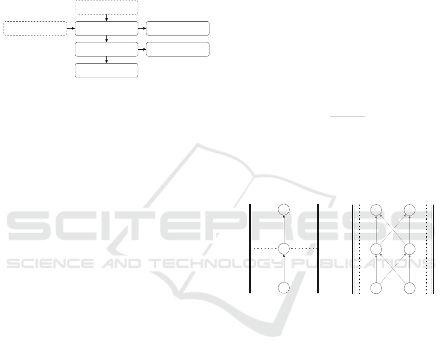
Figure 1: Overview of system architecture.
Our proposed system is made of three main compo-
nents as shown in Figure 1: the lane constructor, path
finder, and pure pursuit modules, which will be ex-
plained in this section. The offline map component
represents the list of waypoints. The perception mod-
ules use raw sensor data to sense parameters such as
drivable area and the positions and measured veloci-
ties of obstacles. These modules are outside the scope
of this paper, but we assume that we can obtain these
parameters.
3.1 Offline Map
The offline map is a directed graph of GPS coordi-
nates called waypoints. Since the waypoints are con-
nected, they imply a heading. Waypoints are used to
mark a section of the road. Since the lateral position
of the vehicle does not depend on the lateral position
of the waypoint on the road, they should not be used
to mark lanes. Each waypoint is also associated with
the maximum driving speed value for this section of
the road.
Waypoints are loaded from the offline map pro-
gressively with a set look-ahead distance starting
from the current vehicle position.
A point cloud map of the environment is saved
locally, and Normal Distributions Transform (NDT)
matching (Biber and Strasser, 2003) is used to de-
termine the vehicle’s position and velocity within the
map from live LiDAR data.
3.2 Lane Construction
Since waypoints do not carry information about the
road width or lane positions (and not all roads have
clearly defined lanes), we need to be able to construct
our own lane positions for the vehicle.
From drivable area data, we can know the width
of the road at any waypoint position. Since waypoints
have a heading, we can construct a line at the way-
point position normal to the waypoint heading. This
line will intersect with the boundaries of the driv-
able area of the road. The road width is then calcu-
lated as the distance between the leftmost and right-
most points of intersection along the constructed line,
shown in Figure 2 as W
L
and W
R
respectively.
The road width is used to determine a reasonable
number of lanes at the position of each waypoint.
Given the left and right distances from the waypoint
to the road boundaries W
L
and W
R
respectively, and
the desired lane width L, we can calculate the number
of lanes N as:
N =
W
L
+W
R
L
(1)
Lanes are centered within the drivable area of the
road, and are not separated by any distance. The new
waypoints are positioned at the center of each con-
structed lane, as shown in Figure 3. These waypoints
are passed to the next step, the path finder module.
N2
N3
N1
W
L
W
R
Figure 2: Calculation of
road width W at the way-
point N2.
N1
N2
N3
N1
N2
N3
Figure 3: Constructed lane
waypoints.
3.3 Assigning Costs
A cost value in the interval [0, 1] is assigned to each
lane waypoint. These values are primarily assigned
according to the proximity of nearby obstacles. A
waypoint having a cost of 1 is considered to be im-
passable.
The cost of a waypoint can be interpreted as the
measured risk of driving through it. A waypoint hav-
ing a cost closer to 1 is likely to be in close vicinity
of one or more obstacles. As a safety measure, the
speed of the vehicle is linked to the waypoint cost: as
the cost approaches 1, the driving speed approaches
0. Thus, if V
T
is the target driving speed, V
W
is the
maximum speed set to the current waypoint, and C is
the waypoint cost, the target speed can be expressed
as:
Path Planning for Autonomous Vehicles with Dynamic Lane Mapping and Obstacle Avoidance
433

V
T
= V
W
∗ (1 − C) (2)
3.3.1 Static Obstacles
Static obstacles are modeled as circular regions hav-
ing a position and a radius. Lane waypoints are also
assigned a circular region having a diameter equal to
the lane width, as shown in Figure 4. If the obstacle
region interesects the waypoint region, the waypoint
is assigned a cost of 1.
Since the waypoint region covers the width of the
lane, and practically the distance between consecutive
waypoints will be very small, a lane that intersects an
obstacle will always be blocked.
N1
N2
N3
N1
N2
N3
Figure 4: A static obstacle, shown as a solid gray circle,
intersects the regions of the N2 lane waypoints.
3.3.2 Moving Obstacles
Moving obstacles are modeled as a single point in
space having a velocity vector. Obstacles are expected
to follow this vector at constant velocity. Changes in
the velocity of an obstacle can only be accounted for
at the next planning interval, after the velocity vector
is updated.
To find the possibility of collision with a moving
obstacle at a given waypoint, a velocity vector for
each waypoint is defined to be a vector pointing in
the same heading as the waypoint and having a mag-
nitude equal to the current vehicle speed.
To determine for a given waypoint whether the
chance of collision with a moving obstacle exists
within a defined time frame, we obtain the paramet-
ric equations for the moving obstacle and the vehicle
driving along the waypoint velocity vector. We are in-
terested in finding two parameters t
ob
and t
wp
, the time
parameters for the obstacle and waypoint equations
respectively, that result in the equality of the position
vectors of the vehicle and waypoint. A solvable sys-
tem indicates that the two constructed straight lines
intersect. Furthermore, if the magnitude in difference
between the two parameters t
ob
and t
wp
is within a
defined range, this indicates that the obstacle and the
vehicle will pass through the same point in space at
nearly the same time. This range can depend on the
physical size of the vehicle and the separation dis-
tance required.
This process is repeated for each waypoint and
moving obstacle pair. A waypoint whose check fails
with any of the detected moving obstacles (i.e. the
difference in the parameters t
ob
and t
wp
is too small)
is assigned a cost of 1.
3.3.3 Cost Smoothing
The techniques described so far can detect whether
a waypoint is in direct contact with an obstacle, or
in the path of a moving obstacle. In both cases, the
waypoint should be completely blocked. Thus, we
can only assign waypoints a cost of 0 or 1 depending
on whether the waypoint intersects with an obstacle.
This can result in paths that are in very close con-
tact to an obstacle when safer alternatives exist. For
example, in Figure 5, the vehicle is initially driving
in the leftmost lane, so it continues to drive in that
lane until the last waypoint that is not in contact with
the obstacle, and then makes a lane switch to the mid-
dle lane right before encountering the obstacle. All
waypoints in the path have a cost of 0, so the vehicle
moves at the maximum allowed speed. In this sce-
nario, the selected path is unfavorable as it moves the
vehicle dangerously close to an obstacle at possibly
high speeds.
We can represent the costs in the grid of waypoints
in Figure 5 by the following 2D matrix:
W =
1.0 0.0 0.0
1.0 0.0 0.0
0.0 0.0 0.0
0.0 0.0 0.0
0.0 0.0 0.0
0.0 0.0 0.0
0.0 0.0 0.0
(3)
In order to achieve a cost gradient, a discrete 2D con-
volution is used. This kernel is used in the simulation:
K =
0.1 0.5 0.1
0.2 1.0 0.2
0.2 0.5 0.2
0.1 0.3 0.1
0.0 0.2 0.0
0.0 0.1 0.0
0.0 0.1 0.0
(4)
K
22
is the center of the kernel. For edge cells, zero
padding is used. All values of the output matrix are
ICAART 2021 - 13th International Conference on Agents and Artificial Intelligence
434
bound to [0, 1]. The kernel values are selected to in-
troduce a cost to the waypoints leading to the obsta-
cle, the first waypoint ahead of the obstacle, and the
lanes adjacent to the blocked lane. Changing these
values effectively changes the obstacle avoidance pro-
file of the vehicle. For example, increasing the val-
ues will cause the vehicle to decelerate more sharply
when approaching an obstacle, favoring safety versus
comfortability. The matrix size determines the dis-
tance from the obstacle at which the vehicle starts the
avoidance maneuver.
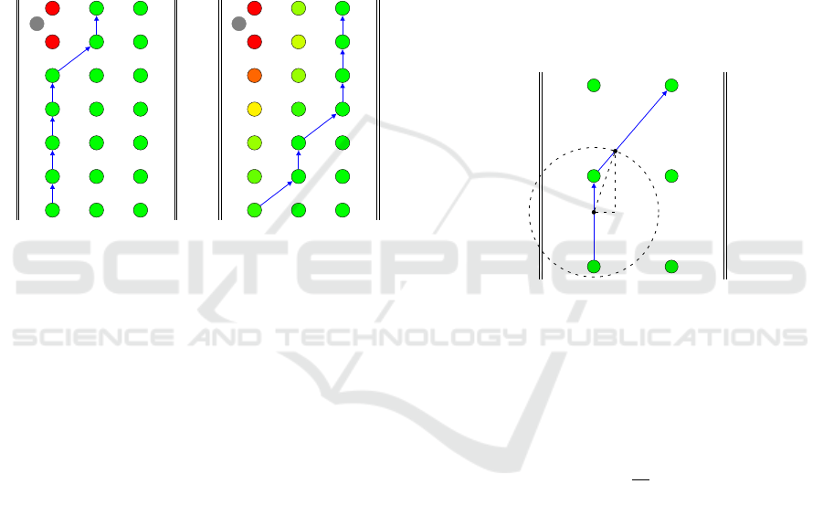
Figure 6 shows the generated path after using the
costs from the W ∗ K matrix on the waypoint grid.
S
Figure 5: Generated path
in a 3-lane road with
a static obstacle, without
cost smoothing.
S
Figure 6: Generated path
after cost smoothing.
3.4 Path Finding
The best path in a lane waypoint grid is modeled as
a shortest path problem. As shown in Figure 3, lane
waypoints can be modeled as a directed graph where
each node connects to the next node in the same lane,
and the next nodes in the left and right lanes signify-
ing a lane change.
The D* lite algorithm (Koenig and Likhachev,
2002) is used to find the shortest path between the
current waypoint and any of the goal waypoints. Goal
waypoints are the final set of lane waypoints in the
loaded section of the offline map.
To decrease the number of lane changes, a con-
stant value is added to the traversal cost when making
a lane change. As a result, the planner will not make a
lane change unless the difference between the cost of
the current lane waypoint and the target lane waypoint
is greater than a certain constant value.
3.5 Vehicle Trajectory
An implementation of the pure pursuit algorithm
(Coulter, 1992) is used to steer the vehicle along the
generated path. Pure pursuit finds a curvature that
moves the vehicle from its current position to a goal
position. The goal position is calculated by construct-
ing a circle with a defined search radius centered
around the vehicle position. Then, a straight line is
constructed between each two consecutive waypoints.
The intersection point between the search circle and
the first line that intersects it is set to be the goal way-
point.
The search radius is typically a function of the cur-
rent vehicle speed. The changes in vehicle heading
become steeper as the search radius decreases. For
purposes of the simulation, it is set to the vehicle
speed multiplied by 2.5, as this value was found in
testing to result in smooth steering curves while not
deviating too far away from the waypoint plan during
turns.
V
T
l
x
Figure 7: Pure pursuit target construction.
The goal is to find the radius of the circle that joins the
vehicle position V with the target point T , such that
the chord length from V to T is equal to the search
radius l. The radius can be expressed as: (Coulter,
1992)
r =
l
2
2x
(5)
The arc joining V and T with radius r is the final in-
tended trajectory of the vehicle.
4 PERFORMANCE EVALUATION
4.1 Simulation Experiments
The LGSVL Simulator provides an environment for
testing autonomous driving functionalities in a 3D en-
vironment. The simulator integrates with the ROS
platform, providing a vehicle model which can be
controlled using ROS commands, and simulates sen-
sors typically used in autonomous driving such as
camera, LiDAR and GPS.
Path Planning for Autonomous Vehicles with Dynamic Lane Mapping and Obstacle Avoidance
435
The simulator was used to test the static and mov-
ing obstacle avoidance capabilities of the proposed
system by two means: Simulating a static obstacle
ahead of the vehicle position in the same driving lane,
and simulating a moving obstacle moving laterally in
front of the vehicle (i.e. a person crossing the road).
The distance from the obstacle to the vehicle and the
deceleration of the vehicle are evaluated.
The test route is a straight 4-lane road section 556
meters long, with a single turn. The target speed for
the test was set to 25 km/h. Higher speeds were not
tested due to technical constraints of the simulation
environment.
4.1.1 Results of the Simulation Test
During the test, the vehicle managed to stay within a
safe distance from all introduced obstacles.
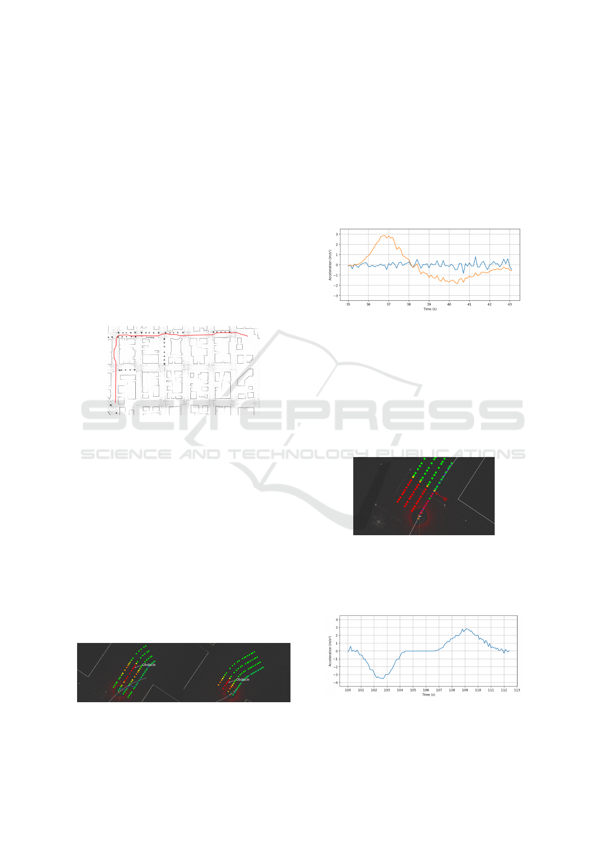
Figure 8: Vehicle path within a point cloud map of the en-
vironment.
In the static obstacle tests, the vehicle initiated a lane
change approximately 14 meters away from the obsta-
cle. Figure 9 shows the maneuver made by the vehi-
cle as the obstacle comes into the look-ahead distance
of the planner. The vehicle changes to the first lane
from the third lane, and continues driving in the third
lane until encountering the next obstacle. The reason
for the double lane change is due to the configura-
tion of the convolution matrix described in Section
3.3.3, which assigns a cost to the lanes adjacent to
the obstacle. Since the vehicle does not drive into the
higher cost region (shown as the yellow and orange
waypoints in Figure 9), the vehicle’s driving speed
stays constant at 25 km/h for the duration of the lane
change.
Figure 9: Vehicle trajectory at different frames during static
obstacle avoidance, showing the waypoint plan (blue line)
and the pure pursuit trajectory (white arc).
The forward and lateral acceleration (shown in
Figure 10) of the vehicle was recorded during the
maneuver. The lateral acceleration reaches a peak
value of 2.88 m/s
2
(0.29g) when initiating the lane
change, and then reaches 1.84 m/s
2
(0.19g) in the op-
posite direction as the vehicle returns to its forward
position. To ensure the lateral stability of the vehi-
cle in lane changes the lateral acceleration should not
be above 0.4g (Sun and Wang, 2020), which the pro-
posed model does not exceed.
Figure 10: Graph of the forward (blue) and lateral (orange)
acceleration of the vehicle during static obstacle avoidance.
In the moving obstacle tests, a moving obstacle mod-
els a pedestrian crossing the road. Since the direction
of movement of the obstacle is lateral to the road, all
lines are blocked (shown in Figure 11), and the vehi-
cle needs to stop completely. The vehicle reaches a
full stop 10 meters away from the obstacle’s line of
motion, and then begins to accelerate after the obsta-
cle passes the vehicle’s lane.
Figure 11: Waypoint map during a moving obstacle test.
Figure 12 shows the acceleration of the vehicle as it
encounters the moving obstacle, while the vehicle is
stopped, and as it continues its route.
Figure 12: Graph of the forward acceleration of the vehicle
during moving obstacle avoidance.
ICAART 2021 - 13th International Conference on Agents and Artificial Intelligence
436
4.2 Field Test
A live demo of the path planning modules was per-
formed using a modified electric golf cart. Data pro-
cessing and vehicle control is done locally on a com-
puter running the ROS platform. The steering column
and throttle actuators of the vehicle are electrically
connected to an Arduino controller, which receives
commands from a ROS node running on the vehicle
computer through a serial connection.
The steering angle is set to the curvature of the
pure pursuit arc described in Section 3.5. The throttle
value is initially set to 0, and a change to the throt-
tle value is calculated every interval which is propor-
tional to the difference between the target and current
velocities. A full stop of the vehicle is performed by
setting the throttle value to 0. Engine braking assists
in stopping the vehicle in a distance that is sufficiently
short for purposes of the demo.
4.2.1 Mapping
A point cloud map of the testing area was created
using LiDAR mapping, and waypoints were mapped
tracing the testing route. The waypoints were placed
1 meter apart. The route is approximately 175 meters
in length. The route includes a straight section, then
a short slightly uphill climb, followed by a series of
sharp turns. The target speed for the route was set
to 7 km/h as a safety precaution, due to the multiple
turns in the path and to minimize the risk of collision.
The route has a single lane due to space constraints of
the testing area.
4.2.2 Results of the Field Test
Two trials were performed: A first trial where the ve-
hicle makes a full route with no obstacles, and a sec-
ond trial with a simulated pedestrian crossing event
once the vehicle reaches the target speed. The vehi-
cle’s position, heading and velocity data was recorded
for the duration of the two runs.
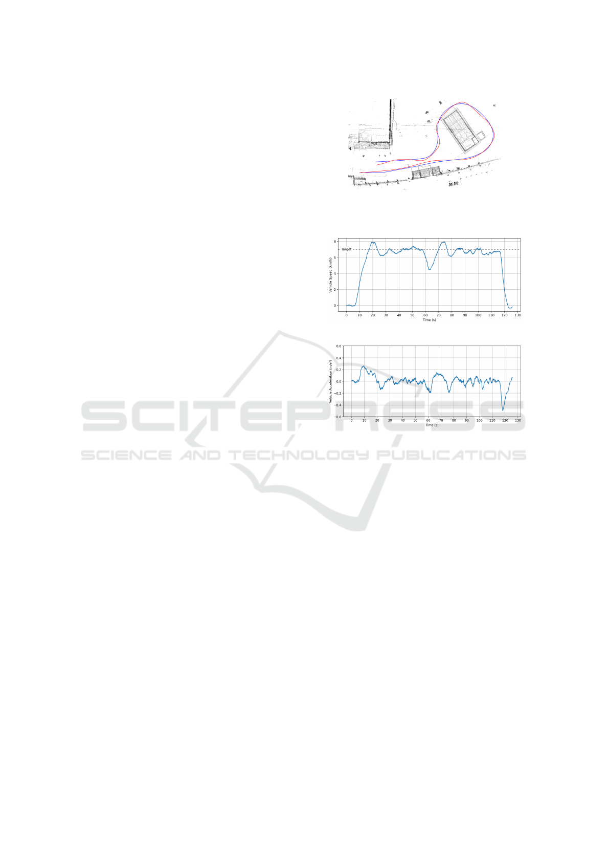
In the first run, the vehicle managed to maneu-
ver around the sharp corners, however it had prob-
lems maintaining its heading in the straight sections,
as shown in Figure 13. This was found to be due to
inaccuracies related to the steering controller of the
vehicle for small steering angles (up to 10 degrees).
Figure 14 shows the vehicle speed for the dura-
tion of the first trial. The vehicle takes 10 seconds to
accelerate to the target speed of 7 km/h. The speed
slightly fluctuates between 6 and 8 km/h (1 km/h de-
viation) for several seconds following accelerating.
This can be resolved by further tuning of the throttle
Figure 13: Actual vehicle path of the test route (red line)
versus the waypoint map (blue line) within a point cloud
map of the first trial.
(a) Vehicle speed
(b) Vehicle acceleration
Figure 14: Vehicle speed and acceleration graphs for the
first trial (no obstacles).
controller of the vehicle. The speed drops at approx-
imately t = 58 s when the vehicle reaches the uphill
part of the route, then the vehicle slowly accelerates
back to its target speed.
The acceleration of the vehicle reaches a maxi-
mum of 0.25 m/s
2
when accelerating from a stopping
position to the target speed, and a minimum of -0.5
m/s
2
when stopping at the end of the route.
For the second trial, three pedestrian crossing
events were initiated at t = 11 s, 41 s, and 59 s dur-
ing the test. The speed and acceleration of the vehi-
cle (shown in Figure 15) were recorded for the dura-
tion of the trial. In each event, a simulated obstacle
was placed 7 meters ahead of the current position in
the path of the vehicle and removed several seconds
later. The distance between the vehicle and the ob-
stacle position was recorded, shown in Figure 15 (b).
The vehicle starts to decelerate as soon as the obstacle
is detected and manages to stop an average of about 3
meters away of the obstacle in the three events.
Path Planning for Autonomous Vehicles with Dynamic Lane Mapping and Obstacle Avoidance
437
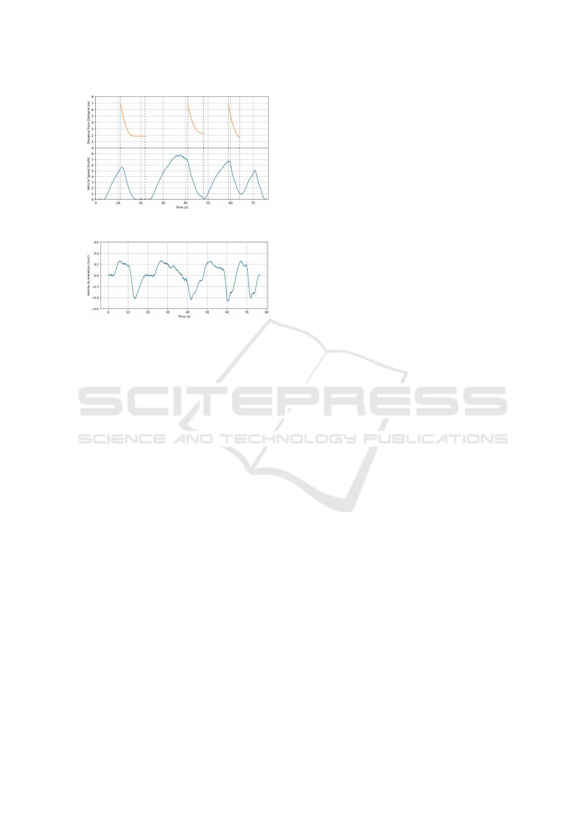
(a) Distance between vehicle and obstacle in meters
plotted against the current vehicle speed in km/h
(b) Vehicle acceleration
Figure 15: Vehicle speed and acceleration graphs for the
second trial (obstacle testing).
5 CONCLUSIONS
In this paper, we present a novel path planning ap-
proach with static and moving obstacle avoidance,
and dynamic lane mapping from road width calcu-
lated from real-time drivable area data. We evaluate
our approach by means of a simulation test, as well
as a real world demo by implementing and running
the model on a vehicle modified to allow autonomous
driving functionalities.
The proposed model was tested on speeds of up to
25 km/h. Thus, further testing needs to be performed
in order to verify the validity of the model with higher
speeds. A limitation in the approach is that the con-
volution matrix described in Section 3.3.3 is static, so
the separation distance between the vehicle and sur-
rounding obstacles does not change depending on the
driving speed. Such limitation would pose safety risks
when driving at high speeds. Therefore, the convolu-
tion approach needs to be adjusted with high speed
driving taken into consideration. Moreover, the pro-
posed approach needs to be improved to find the in-
tersection between obstacles and waypoints, as it may
not cover cases where an obstacle is positioned in cer-
tain positions of the road outside the waypoint region
but still posing a risk to the vehicle. Finally, a confir-
mation window for the drivable area needs to be im-
plemented in order to account for short variations in
drivable area width and the number of lane waypoints.
REFERENCES
Ahmed, A. A., Abdalla, T. Y., and Abed, A. A. (2015). Path
planning of mobile robot by using modified optimized
potential field method. International Journal of Com-
puter Applications, 113:6–10.
Biber, P. and Strasser, W. (2003). The normal distributions
transform: A new approach to laser scan matching. In
Proceedings of the 2003 IEE/RSJ International Con-
ference on Intelligent Robots and Systems.
Boroujeni, Z., Goehring, D., Ulbrich, F., Neumann, D.,
and Rojas, R. (2017). Flexible unit a-star trajectory
planning for autonomous vehicles on structured road
maps. 2017 IEEE International Conference on Vehic-
ular Electronics and Safety (ICVES), pages 7–12.
Coulter, R. C. (1992). Implementation of the pure pursuit
path tracking algorithm. Technical Report CMU-RI-
TR-92-0, Camegie Mellon University.
Daily, R. and Bevly, D. M. (2008). Harmonic potential field
path planning for high speed vehicles. In 2008 Amer-
ican Control Conference, pages 4609–4614.
Elbanhawi, M., Simic, M., and Jazar, R. (2015). In the
passenger seat: Investigating ride comfort measures
in autonomous cars. IEEE Intelligent Transportation
Systems Magazine, 7:4–17.
Francis, S. L., Anavatti, S. G., and Garratt, M. (2018). Real-
time path planning module for autonomous vehicles
in cluttered environment using a 3d camera. Int. J.
Vehicle Autonomous Systems, 14:40–61.
Hu, X., Chen, L., Tang, B., Cao, D., and He, H. (2018). Dy-
namic path planning for autonomous driving on var-
ious roads with avoidance of static and moving ob-
stacles. Mechanical Systems and Signal Processing,
100:482–500.
Koenig, S. and Likhachev, M. (2002). D* lite. In Proceed-
ings of the Eighteenth National Conference on Artifi-
cial Intelligence.
Lemos, R., Garcia, O., and Ferreira, J. V. (2016). Local and
global path generation for autonomous vehicles using
splines. Ingenier
˜
Aa, 21:188–200.
Montemerlo, M., Becker, J., Bhat, S., Dahlkamp, H., Dol-
gov, D., Ettinger, S., Haehnel, D., Hilden, T., Hoff-
mann, G., Huhnke, B., Johnston, D., Klumpp, S.,
Langer, D., Levandowski, A., Levinson, J., Marcil, J.,
Orenstein, D., Paefgen, J., Penny, I., Petrovskaya, A.,
Pflueger, M., Stanek, G., Stavens, D., Vogt, A., and
Thrun, S. (2008). Junior: The stanford entry in the
urban challenge. Journal of Field Robotics, 25:569–
597.
Sun, W. and Wang, S. (2020). Research on lateral acceler-
ation of lane changing. International Conference on
Frontier Computing, pages 950–960.
WHO (2020). Road traffic injuries.
https://www.who.int/news-room/fact-
sheets/detail/road-traffic-injuries. Accessed: 2020-
07-29.
Zhang, S., Deng, W., Zhao, Q., Sun, H., and Litkouhi, B.
(2013). Dynamic trajectory planning for vehicle au-
tonomous driving. 2013 IEEE International Confer-
ence on Systems, Man, and Cybernetics, pages 4161–
4166.
ICAART 2021 - 13th International Conference on Agents and Artificial Intelligence
438
