Quantification of Uncertainty in Brain Tumor Segmentation using
Generative Network and Bayesian Active Learning
Rasha Alshehhi
1
and Anood Alshehhi
2
1
New York University Abu Dhabi, U.A.E.
2
Tawam Hospital, Al Ain, U.A.E.
Keywords:
Segmentation, Generative Adversarial Network, Uncertainty, Bayesian Active Learning.
Abstract:
Convolutional neural networks have shown great potential in medical segmentation problems, such as brain-
tumor segmentation. However, little consideration has been given to generative adversarial networks and
uncertainty quantification over the output images. In this paper, we use the generative adversarial network
to handle limited labeled images. We also quantify the modeling uncertainty by utilizing Bayesian active
learning to reduce untoward outcomes. Bayesian active learning is dependent on selecting uncertain images
using acquisition functions to increase accuracy. We introduce supervised acquisition functions based on
distance functions between ground-truth and predicted images to quantify segmentation uncertainty. We
evaluate the method by comparing it with the state-of-the-art methods based on Dice score, Hausdorff distance
and sensitivity. We demonstrate that the proposed method achieves higher or comparable performance to
state-of-the-art methods for brain tumor segmentation (on BraTS 2017, BraTS 2018 and BraTS 2019 datasets).
1 INTRODUCTION
Convolutional neural networks (CNNs) have been
shown to outperform other segmentation methods in
different medical applications (e.g., blood vessels,
brain-tumor and lung). Mainly, most previous works
focus on maximizing accuracy and less attention has
been given to evaluate uncertainty quantification in the
network outputs. It is essential to measure uncertainty
in medical applications to understand the reliability
of the segmentation and identify challenging cases ne-
cessitating expert review. On the other hand, neural
networks are subject to over-fitting and pixel-based
prediction may provide incorrect classification with
spurious high confidence.
Many previous works use Bayesian modeling to
measure epistemic or aleatoric uncertainty. Epis-
temic is a result of uncertainty in the model param-
eters, which can be avoided with given enough data.
Aleatoric is a result of noise inherent in the input data
(e.g., sensor noise and motion) and unaffected by the
amount of available data. There are two categories of
aleatoric uncertainty. The first category is homoscedas-
tic uncertainty, which is constant with different inputs.
The second category is heteroscedastic uncertainty,
which varies with different inputs (Kendall and Gal,
2017).
In this work, we use the generative adversarial
model (GAN) (Goodfellow et al., 2014). The GAN per-
forms well with unlabeled samples (unsupervised) or a
limited number of labeled samples (semi-supervised).
As it is known, the labeled samples are often in-
sufficient in medical applications, difficult to obtain
and annotating a large number of samples is time-
consuming (Xue et al., 2018). We also utilize Bayesian
deep active learning to minimize epistemic uncertainty
in medical segmentation. In Bayesian deep active
learning, we train a model on a small amount of data
(training dataset). We use different acquisition func-
tions that mainly select the most informative samples
from a large dataset (pooling dataset). Then, we add
selected samples to the previous training dataset and
build a new model with the latest training dataset.
This process is repeated and the training dataset is
increased in size with time (Gal et al., 2017). The
primary purpose of active learning is to achieve higher
accuracy with fewer training samples. There are differ-
ent well-known acquisition functions frequently used,
such as random (baseline), entropy, margin sampling
and least confidence (Wang et al., 2017). These func-
tions usually select informative samples relying on the
probability estimation (unsupervised functions). In
this work, we introduce new supervised acquisition
functions based on distance functions between ground-
Alshehhi, R. and Alshehhi, A.
Quantification of Uncertainty in Brain Tumor Segmentation using Generative Network and Bayesian Active Learning.
DOI: 10.5220/0010341007010709
In Proceedings of the 16th International Joint Conference on Computer Vision, Imaging and Computer Graphics Theory and Applications (VISIGRAPP 2021) - Volume 4: VISAPP, pages
701-709
ISBN: 978-989-758-488-6
Copyright
c
 2021 by SCITEPRESS – Science and Technology Publications, Lda. All rights reserved
701

truth and predicted images: Jaccard, Hausdorff and
maximum mean discrepancy (MMD) distances.
This paper is organized as follows. Section 2 shows
some previous works used for brain-tumor segmen-
tation: generative adversarial networks and convolu-
tional neural networks with uncertainty functions. Sec-
tion 3 presents our contributions. Section 4 presents
the proposed generative model and Bayesian active
learning highlighting new acquisition functions. Ex-
perimental results are demonstrated in Section 5. Sec-
tion 6 summarizes this work.
2 RELATED WORK
In this section, we present the previous works for
brain-tumor segmentation that uses generative net-
works (Section 2.1) and Bayesian deep learning (Sec-
tion 2.2).
2.1 Generative Adversarial Networks
Some works used generative networks for brain-tumor
segmentation. Xue et al. (Xue et al., 2018) was the
first authors who proposed a novel end-to-end adver-
sarial neural network, called SegAN. They used a
fully-convolutional neural network as a generator and
discriminator with a multi-scale L1 loss function to
learn spatial detail. Giacomello et al. (Giacomello
et al., 2019) extended the previous network SegAN
by adding Dice Score to the multi-scale L1 loss func-
tion, call SegAN-CAT. However, both works did not
estimate the uncertainty of the brain-tumor structure.
2.2 Bayesian Active Learning
As we pointed out previously, uncertainty information
is a result of the input data (aleatoric estimation) or
model (epistemic estimation). Most previous works
focused on epistemic assessment. Gal et al. (Gal et al.,
2017) introduced cost-effective selection strategies to
Bayesian deep active learning to estimate model un-
certainty with high accuracy and less manual anno-
tations. This method achieves promising results in
classification problems. However, it is computation-
ally expensive. Kendall and Gal (Kendall and Gal,
2017) combined aleatoric and epistemic uncertainty
estimates in Bayesian deep learning for both regres-
sion and classification applications. Their methods has
ideal performance with noisy data.
There are many studies (Eaton-Rosen et al., 2018;
Jungo et al., 2018; Wang et al., 2019a; Wang et al.,
2019b) utilized medical uncertainty based either on
aleatoric or epistemic estimations, but none of them
use Bayesian deep active learning. Wang et al. (Wang
et al., 2019a) used a combination of aleatoric and epis-
temic to estimate uncertainties for whole tumor seg-
mentation. Wang et al. (Wang et al., 2019b) also
proposed a cascade of hierarchical CNNs to segment
all brain-tumor structures, unlike (Wang et al., 2019a),
and used test-time augmentation to obtain not only
segmentation outputs but also data-based uncertainty
(aleatoric) of all structures of brain-tumor segmenta-
tion.
3 CONTRIBUTION
In this work, we use Bayesian deep active learning
to estimate the model uncertainty (epistemic) of all
brain-tumor structures. Few works address uncer-
tainty in all structures of brain-tumor (e.g., cascade
CNNs (Wang et al., 2019b)). We train generative net-
works with small datasets, use active learning to query
more samples using well-known acquisition functions
introduced in (Wang et al., 2017) such as entropy, mar-
gin sampling, least confidence and random sampling.
Usually, active learning is used to query samples with
the most informative samples because of limited la-
beled samples. We introduce three acquisition super-
vised functions dependent on pixel-to-pixel distances
between each brain-tumor structure of both ground-
truth and predicted image. We estimate pixel-to-pixel
distances and select samples based on the average
distance. The distances are Jaccard, Hausdorff and
maximum mean discrepancy (MMD) distances.
4 METHOD
This section illustrates the proposed method. It is
based on applying Bayesian active learning to the gen-
erative adversarial network by selecting uncertain sam-
ples and updating the generative model for brain-tumor
segmentation. Figure 1 represents an overview of the
proposed method.
4.1 Generative Adversarial Network
(Figure 1 - I)
Deep generative adversarial network (GAN) (Good-
fellow et al., 2014; Isola et al., 2017) is a two-player
min-max game. It consists of a generator and a dis-
criminator. The generator ( G ) captures the data dis-
tribution of the real image and produces a synthetic
label image. The discriminator ( D ) differentiates the
data distribution of the true label image from the data
VISAPP 2021 - 16th International Conference on Computer Vision Theory and Applications
702

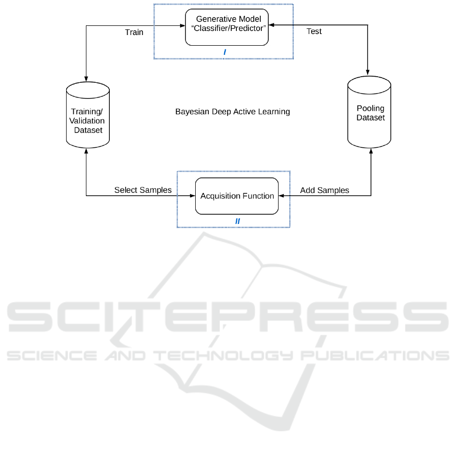
Figure 1: An overview of Bayesian deep active learning. It consists of the following processes: (A) Train the generative model
on the training dataset, (B) Test model on a subset of the pooling dataset, (C) Apply unsupervised/ supervised acquisition
function on samples and (D) Select samples to add to training dataset and rebuild a new generative model.
distribution of the generator’s output label image. The
generator and discriminator combat with each other in
the training step to minimize an objective function:
G
?
= argmin
G
max
D
L
cGAN
(G, D) + λL
l2
(G),
(1)
where L
cGAN
(G, D) is a conditional loss of the gener-
ative adversarial model and L
l2
(G) is a mean square
error between true label image and generated label
image.
L
cGAN
(G, D) =
E
y∼P
r
[log(D(x, y)] + E
G(x)∼P
f
[log(1 − D(x, G(x)))] ,
(2)
L
l2
(G) = E
y∼P
r
,G(x)∼P
f
[||y − G(x)||
2
],
(3)
where P
r
is the real data distribution and P
f
is the
fake data distribution (generated). x and y are input
images and true label images. G(x) = ˆy is an output
label image from the generator. We use uNet with
ResNet architecture (He et al., 2016) as a generator.
It consists of 8 convolution blocks, which consist of
convolution, batch normalization and LeaklyReLU ac-
tivation. It also consists of 8 deconvolution blocks,
consisting of deconvolution, batch normalization and
ReLU activation, and skip-connection. It starts with
64 filter kernels of size (4 × 4) . The discriminator net-
work D also has the same architecture. It consists of
8 convolution blocks. Each block consists of convolu-
tion, batch normalization and LeaklyReLU activation,
starting with 64 kernels of size (4 × 4) . The last layer
of convolution is connected with a sigmoid function
to generate a distribution map of each class.
4.2 Bayesian Active Learning
The previous network is trained under the Bayesian
active learning framework (Gal et al., 2017; Kendall
and Gal, 2017). Suppose we use a dataset D
total
of N
samples and C classes:
D
total
=
{
(x
0
, y
0
), (x
1
, y
1
), (x
2
, y
2
), ..., (x
N−1
, y
N−1
)
}
(4)
We divide D
total
into initial training dataset D
train
,
pooling dataset D
pool
and validation dataset D
valid
.
We start with the initial training dataset D
train
, vali-
date with validation data D
valid
. The training dataset
incremental grows by selecting samples from D
pool
based on selection functions called acquisition func-
tions (Figure 1 - II), which we will discuss in detail in
this section. The main objective of Bayesian deep ac-
tive learning is to minimize loss function and improve
accuracy.
We fix generative network parameters W . We rank
all samples according to the two types of criteria: su-
pervised and unsupervised. The supervised criteria are
Jaccard, Hausdorff and MMD distances. The unsuper-
vised criteria are entropy, margin sampling and least
confidence (Gal et al., 2017; Wang et al., 2017). After
initial training, we test the model M with subset of
pooling data D
pool
for T
pool
times and select L most
uncertain samples from D
pool
based on selection func-
Quantification of Uncertainty in Brain Tumor Segmentation using Generative Network and Bayesian Active Learning
703

tions to add to training dataset D
train
. This process
is repeated for T
train
. The most uncertain ones in the
supervised selection approach are with maximum dis-
tances between ground-truth y and predicted outputs
ˆy . However, the most uncertain ones in the unsuper-
vised selection approach are with maximum entropy,
minimum margin and minimum least confidence.
The supervised selection criteria are based on the
maximum pixel to pixel distance between true and
predicted images:
• Jaccard distance: it is used as an evaluation metric
in segmentation problems. Here we rank samples
in D
pool
in a descending order and select samples
of largest distances (more uncertain ones) to add
to D
train
according to:
J(y, ˆy) =
1
C
C
∑
c=1
y
c
∩ ˆy
c
y
c
+ ˆy
c
− (y
c
∩ ˆy
c
)
, (5)
• Hausdorff distance: it is the maximum distance
of all pixels from ground-truth image to the cor-
responding nearest pixel of the predicted segmen-
tation image. Mainly, this distance is used as an
evaluation metric or loss function (Isensee et al.,
2017; Sauwen et al., 2017). Here we rank samples
in D
pool
in a descending order and select samples
of largest distances to add to D
train
according to:
H(y, ˆy) =
1
C
C
∑
c=1
(
1
N
y
c
∑
v∈y
c
min
w∈ ˆy
c
k
w − v
k
2
+
1
N
ˆy
c
∑
w∈ ˆy
c
min
v∈y
c
k
w − v
k
2
),
(6)
where N
y
c
and N
ˆy
c
are the number of pixels in
ground-truth image y and predicted image ˆy of
class c.
• Maximum mean discrepancy (MMD): it is usually
defined as a distance between two distributions
Q
y
and Q
ˆy
(Sutherland et al., 2017). Here, we
rank samples in D
pool
in an descending order and
select samples of largest distances to add to D
train
according to:
MMD(Q
y
, Q
ˆy
) = E
y∼Q
y
(y) − E
ˆy∼Q
ˆy
( ˆy), (7)
MMD(Q
y
, Q
ˆy
) =
1
C
C
∑
c=1
(
∑
i6= j
K(y
i
, y
j
)
−
∑
i6= j
K(y
i
, ˆy
j
) +
∑
i, j
K( ˆy
j
, ˆy
j
)),
(8)
where K(y
i
, y
j
) = ky
i
− y
j
k
2
; i and j are pixels ei-
ther on ground-truth image y or predicted image
ˆy . K(y
i
, y
j
) and K( ˆy
i
, ˆy
j
) show within distribution
similarity; however, K(y
i
, ˆy
j
) show cross distribu-
tion similarity.
We also use in conjunction with previous methods,
unsupervised criteria from (Gal et al., 2017; Wang
et al., 2017). The selection is based on probability of
pixel x belonging to the class c P(y = c|x;W ) ; where
c is the index of class:
• Entropy: we rank samples in a descending order.
The higher entropy sample is more uncertain one:
EN(y) = −
C
∑
c=1
P(y = c|x;W ) × logP(y = c|x;W ),
(9)
• Margin sampling: we rank samples based on the
first (a) and second (b) most probability class pre-
dicted by the model. The smaller margin means
more uncertain.
MS(y) = P(y
i
= c
a
|x;W )−P(y
i
= c
b
|x;W ), (10)
• Least confidence: we rank samples in an ascend-
ing order. The lower least confidence is the more
uncertain one.
LC(y) = max
c
P(y = c|x;W ), (11)
5 EXPERIMENTAL
PERFORMANCE
In the previous section, we present the proposed
method highlighting acquisition functions, which will
measure the generative network’s uncertainty. In this
section, we illustrate the performance of the genera-
tive networks with various query functions. Section 5.1
and Section 5.2 present used data, setting and evalu-
ation metrics. Section 5.3 shows some results of the
proposed method compared to other methods.
5.1 Data
We use datasets of medical image computing and
computer-assisted intervention (MICCAI) of multi-
modal brain-tumor segmentation (BraTS) Challenge
2017, 2018 and 2019 (Bakas et al., 2017; Menze et al.,
2015). The BraTS 2017 and BraTS 2018 share the
same dataset. It comprises 285 multi-institutional pre-
operative multi-modal magnetic resonance imaging
(MRI) scans glioblastoma (GBM/HGG) (210 scans)
and lower-grade glioma (LGG) (75 scans). The BraTS
2019 consists of a total of 335 MRI volumes (259
HGG and 76 LGG). The BraTS data is available in
(https://www.med.upenn.edu/sbia/) and (https://www.
med.upenn.edu/cbica/). Each multi-modal scan con-
sists of native (T1) and post-contrast T1-weighted
(T1Gd), T2-weighted (T2) and T2 Fluid Attenuated
VISAPP 2021 - 16th International Conference on Computer Vision Theory and Applications
704

Inversion Recovery (FLAIR) volumes. Each volume
of size 240 × 240 consists of 155 slices. The ground-
truth volume 240 × 240 × 155 of each scan comprises
of peritumoral edema (ED — label 2), necrotic and
non-enhancing tumor core (NCR/NET — label 1) and
GD-enhancing tumor (ET — label 4). The whole tu-
mor (WT) includes ED, NCR/NET and ET, core tumor
(TC) includes NCR/NET and ET and enhanced tumor
(ET) includes only ET.
5.2 Experimental Setup and Metrics
The dataset of MICCAI BraTS is divided into four
subsets: initial training D
train
(20 samples), validation
D
valid
(30 samples), pooling D
pool
(190 samples for
BraTS 2017-2018 and 240 for BraTS 2019) and test-
ing samples D
test
(45 samples). The training process
is run for 5 times (number of experiments, N
e
= 5 ); at
each experiment ( i
e
), the 3D networks are trained with
initial training set D
train
and evaluate with validation
set D
valid
. At each experiment i
e
, the networks are run
for 10 times (number of queries, N
q
= 10 ). At each
query ( i
q
), the networks are evaluated with a pooling
set for 10 times (Monte Carlo (MC) dropout iterations,
N
d
= 10 ). Based on the results of acquisition functions
in each query ( i
q
), 10 samples are retrieved from pool-
ing set and the networks are retrained using previous
initial training set D
train
and subset of pooling data
D
pool
. We assess the uncertainty in prediction outputs
by applying acquisition functions dependent on proba-
bilities of predicted images (entropy, margin sampling
or least confidence) or distance between ground-truth
and predicted images (jaccard, Hausdorff or MMD).
We compare the proposed method with two con-
volutional networks (Isensee et al., 2017; Myronenko,
2018). We use the same training procedures used in
both works with the same loss functions: Dice coeffi-
cient, L2 and KL. We also compare with state-of-the-
art networks (Jungo et al., 2018; Wang et al., 2019b;
Giacomello et al., 2019; Xue et al., 2018; Mazumdar,
2020) and use the same training procedures with multi-
scale L1 loss and Dice coefficient. We use Disc score,
Hausdorff score and true positive rate (TPR)/sensitivity
to evaluate enhancing tumor (ET), necrotic and non-
enhancing tumor core (NCR/NET) and edema (ED)
structures. We run all experiments on Nvidia Tesla
V100 GPUs-32 GB with Keras 2 of Tensorflow 1.4.
5.3 Results
In this section, we compare the performance of the
proposed method with common convolutional net-
works on BraTS 2017 on BraTS 2018 datasets in Sec-
tion 5.3.1 and Section 5.3.2 and with state-of-the-art
methods on BraTS 2019 in Section 5.3.3.
5.3.1 Comparison the Proposed Method with
Isensee’s Network on BraTS 2017 Dataset
F. Isensee (Isensee et al., 2017) uses uNet architecture
and Dice coefficient as a loss function to cope with
class imbalance. Data augmentation is used to avoid
over-fitting. This work was one of the leading methods
in BraTS 2015 and BraTS 2017.
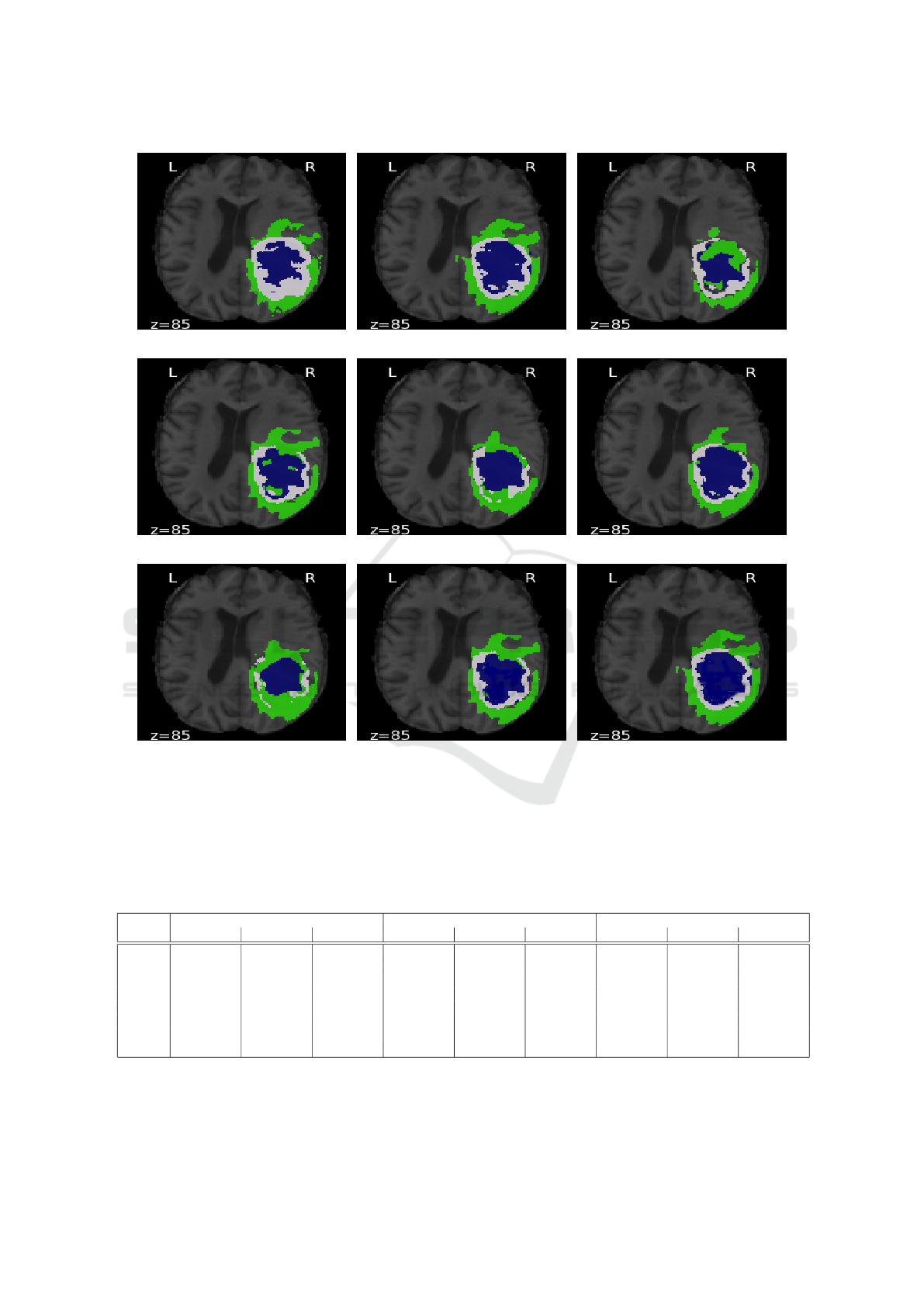
In Figure 2, we compare the results of applying
Isensee’s network (Isensee et al., 2017) and generative
networks with Bayesian active learning utilizing previ-
ous acquisition functions. The predicted images, based
on unsupervised functions random, entropy, margin
sampling and least confidence, show more uncertainty
and overlap sub-regions between ED and NCR/NET
borders and many regions that are potentially seg-
mented incorrectly 2(c)-2(f). The predicted image
based on Jaccard distance 2(g) also shows relatively
higher uncertainty between NCR/NET and ED than
the interior structure (ET). However, predicated im-
ages based on Hausdorff and MMD distances 2(h)-2(i)
have lower uncertainty, in particularity where other
uncertainty maps 2(c)-2(g) mismatches with ground-
truth map 2(a). The uncertainty Hausdorff and MMD
maps identify the previous boundaries with misclassi-
fied some NCR/NET pixels, similar to Isensee’s model
2(b). The prediction uncertainty maps, either super-
vised or unsupervised, reflect a lack of confidence
around boundaries between different classes, which
is changed by increasing the number of experiments,
number of queries, number of MC dropout iterations
or number of training samples in addition to the type
of acquisition function. However, it is computationally
expensive, requiring more time and memory usage.
In Table 1, we compare the results obtained by
previous models on BraTS 2017 dataset. The Dice
score, Hausdorff distance and sensitivity of both su-
pervised and unsupervised methods are comparable.
However, it is remarkable that the networks that ac-
quire samples with Hausdorff distance and then with
MMD distances show low uncertainty and have the
best performance (higher Disc score, lower Hausdorff
distance and higher sensitivity). On the other hand,
uncertainty entropy maps have higher Dice scores and
sensitivity (lower uncertainty) than random, margin
and least-confidence maps.
5.3.2 Comparison the Proposed Method with
Myronenko’s Network on BraTS 2018
Dataset
A. Myronenko (Myronenko, 2018) uses 3D variational
encoder-decoder for automated segmentation of brain-
Quantification of Uncertainty in Brain Tumor Segmentation using Generative Network and Bayesian Active Learning
705

(a) (b) (c)
(d) (e) (f)
(g) (h) (i)
Figure 2: Comparison between predicted images obtained from Isensee’s network and generative network using acquisition
functions: (a) Ground-truth, (b) Isensee (Isensee et al., 2017), (c) Random sampling, (d) Entropy, (e) Margin sampling, (f)
Least confidence, (g) Jaccard, (h) Hausdorff and (i) MMD. Edema (ED) is shown in green, enhancing tumor (ET) in blue and
necrotic and non-enhancing tumor (NCR/NET) in white. z is the index of slice.
Table 1: Comparison between Isensee’s network and generative network with acquisition functions based on Dice, Hausdorff
and sensitivity metrics (mean ± std). RS: random sampling, EN: entropy, MS: margin sampling, LC: least confidence, JD:
Jaccard distance, HD: Hausdorff distance and MMD: MMD distance. WT, TC and ET denote the whole tumor, tumor core and
enhancing tumor.
Method Dice Hausdorff Sensitivity
WT TC ET WT TC ET WT TC ET
Isensee 0.86 ± 0.09 0.59 ± 0.12 0.74 ± 0.12 5.51 ± 2.19 7.52 ± 2.18 2.42 ± 1.38 0.89 ± 0.09 0.62 ± 0.23 0.79 ± 0.19
RS 0.79 ± 0.18 0.52 ± 0.15 0.63 ± 0.15 7.68 ± 2.11 9.69 ± 2.16 7.22 ± 2.12 0.86 ± 0.19 0.59 ± 0.25 0.77 ± 0.23
EN 0.84 ± 0.14 0.53 ± 0.14 0.66 ± 0.12 6.10 ± 2.16 6.49 ± 2.15 6.28 ± 2.15 0.88 ± 0.16 0.59 ± 0.25 0.78 ± 0.23
MS 0.81 ± 0.17 0.80 ± 0.17 0.62 ± 0.11 7.49 ± 2.16 7.71 ± 2.04 8.47 ± 1.24 0.85 ± 0.18 0.58 ± 0.20 0.74 ± 0.20
LC 0.83 ± 0.16 0.54 ± 0.18 0.67 ± 0.18 7.26 ± 2.39 6.68 ± 1.19 5.76 ± 1.84 0.88 ± 0.14 0.59 ± 0.12 0.79 ± 0.13
JD 0.80 ± 0.17 0.56 ± 0.19 0.67 ± 0.13 5.00 ± 2.15 6.02 ± 2.18 4.01 ± 2.85 0.86 ± 0.19 0.61 ± 0.25 0.77 ± 0.11
HD 0.88 ± 0.18 0.62 ± 0.19 0.75 ± 0.12 5.11 ± 2.17 6.11 ± 2.18 4.03 ± 1.15 0.91 ± 0.15 0.64 ± 0.15 0.80 ± 0.14
MMD 0.87 ± 0.17 0.59 ± 0.19 0.73 ± 0.12 5.01 ± 2.17 5.89 ± 2.18 4.83 ± 1.88 0.90 ± 0.19 0.64 ± 0.15 0.79 ± 0.11
VISAPP 2021 - 16th International Conference on Computer Vision Theory and Applications
706

(a) (b) (c)
(d) (e) (f)
(g) (h) (i)
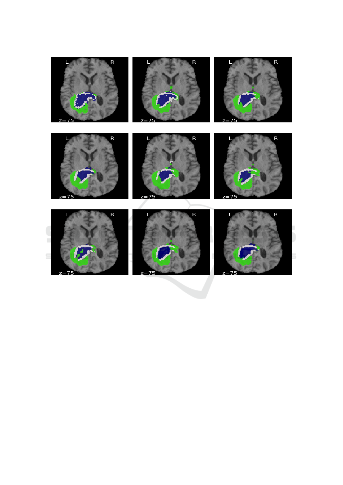
Figure 3: Comparison between predicted images obtained from using Myronenko’s network (Myronenko, 2018) and generative
network with acquisition functions: (a) Ground-Truth, (b) Myronenko, (c) Random sampling, (d) Entropy, (e) Margin sampling,
(f) Least confidence, (g) Jaccard, (h) Hausdorff and (i) MMD. Edema (ED) is shown in green, enhancing tumor (ET) in blue
and necrotic and non-enhancing tumor (NCR/NET) in white. z is the index of slice.
tumor due to limited training data. The author recon-
structs the input image to regularize the decoder and
impose additional constraints on its layers. This work
ranked as 1st place in the BraTS 2018 challenge.
Figure 3 shows an example from the BraTS 2018
dataset. In figure 3(g), the result of the 3D generative
network using Jaccard distance contains some false
positives in ED, NCR/NET and ET regions associated
with higher uncertainties. In contrast, the results of
3D generative networks using Hausdorff and MMD
distances 3(h)-3(i) are smoother, particularly in ET
regions; reflecting lower uncertainty in hierarchical
structures from larger to smaller. On the other hand,
unsupervised functions 3(c)-3(f) show uncertainty in
larger structure (misclassified ED pixels).
We also show obtained results from all unsuper-
vised and supervised methods on BraTS 2018 in Ta-
ble 2. Although Myronenko’s model (Myronenko,
2018) shows a high Dice score, small Hausdorff dis-
tance and high true positive rate, the MMD and then
HD maps show the lowest uncertainty, respectively;
showing a good correlation between uncertainty and
MMD distance or Hausdorff maps. On the other hand,
the network based on entropy has lower uncertainty
outputs than other ground truth independent maps: MS
and LC.
Quantification of Uncertainty in Brain Tumor Segmentation using Generative Network and Bayesian Active Learning
707

Table 2: Comparison between Myronenko’s network and generative network with acquisition functions based on Dice,
Hausdorff and sensitivity metrics (mean ± std). RS: random sampling, EN: entropy, MS: margin sampling, LC: least confidence,
JD: Jaccard distance, HD: Hausdorff distance and MMD: MMD distance. WT, TC and ET denote the whole tumor, tumor core
and enhancing tumor.
Method Dice Hausdorff Sensitivity
WT TC ET WT TC ET WT TC ET
Myronenko 0.90 ± 0.19 0.86 ± 0.12 0.81 ± 0.11 5.51 ± 1.90 6.85 ± 1.11 3.92 ±1.38 0.90 ± 0.11 0.72 ± 0.13 0.80 ± 0.11
RS 0.80 ± 0.18 0.70 ± 0.18 0.60 ± 0.15 8.18 ± 1.99 9.69 ± 1.96 6.22 ± 1.72 0.79 ± 0.11 0.63 ± 0.14 0.71 ± 0.13
EN 0.85 ± 0.13 0.73 ± 0.18 0.72 ± 0.12 6.10 ± 1.76 6.54 ± 1.95 4.28 ± 1.45 0.82 ± 0.16 0.60 ± 0.15 0.72 ± 0.12
MS 0.81 ± 0.16 0.77 ± 0.11 0.71 ± 0.11 7.49 ± 1.76 8.71 ± 1.04 7.41 ±1.42 0.80 ± 0.20 0.61 ± 0.16 0.70 ± 0.17
LC 0.84 ± 0.16 0.70 ± 0.11 0.67 ± 0.12 7.21 ± 1.39 8.05 ± 1.99 5.55 ± 1.84 0.78 ± 0.17 0.62 ± 0.14 0.69 ± 0.11
JD 0.82 ± 0.18 0.74 ± 0.19 0.70 ± 0.14 7.56 ± 1.67 7.69 ± 1.98 5.94 ±1.87 0.85 ± 0.19 0.61 ± 0.15 0.71 ± 0.11
HD 0.91 ± 0.11 0.87 ± 0.15 0.81 ± 0.20 5.56 ± 1.76 5.89 ± 1.95 3.88 ± 1.25 0.90 ± 0.12 0.71 ± 0.15 0.81 ± 0.17
MMD 0.92 ± 0.12 0.88 ± 0.11 0.82 ± 0.21 5.20 ± 1.76 5.01 ± 1.95 3.48 ±1.15 0.93 ± 0.16 0.73 ± 0.12 0.82 ± 0.12
Table 3: Comparison between different CNN architectures based on Dice score and Hausdorff distance (mean ± std). EN and
HD are Entropy and Hausdorff distance. WT, TC and ET denote the whole tumor, tumor core and enhancing tumor.
Method Dice Hausdorff
WT TC ET WT TC ET
CNN+Uncertainty (Jungo et al., 2018) 0.89 ± 0.09 0.78 ± 0.12 0.74 ± 0.28 5.41 ± 1.71 7.48 ± 1.94 5.38 ± 1.07
Cascaded CNN+Uncertainty (Wang et al., 2019b) 0.90 ± 0.05 0.83 ± 0.13 0.78 ± 0.18 6.97 ± 2.56 6.78 ± 2.26 4.28 ± 1.07
Fully Residual CNNs (Mazumdar, 2020) 0.89 ± 0.12 0.82 ± 0.11 0.78 ± 0.12 6.38 ± 1.12 5.91 ± 1.21 4.43 ± 1.12
SegAN (Xue et al., 2018) 0.84 ± 0.12 0.61 ± 0.20 0.64 ± 0.28 7.57 ± 2.33 6.63 ± 1.11 5.60 ± 1.22
SegAN-CAT (Giacomello et al., 2019) 0.86 ± 0.14 0.63 ± 0.20 0.68 ± 0.28 7.79 ± 1.33 6.65 ± 1.11 5.66 ± 1.22
Unsupervised EN 0.87 ± 0.32 0.65 ± 0.12 0.68 ± 0.11 6.51 ± 1.21 6.19 ± 1.15 5.69 ± 1.21
Supervised HD 0.89 ± 0.11 0.82 ± 0.11 0.77 ± 0.17 5.01 ± 1.21 5.21 ± 1.15 4.11 ± 1.15
5.3.3 Comparison the Proposed Method with
State-of-the-Art Methods on BraTS 2019
Dataset
In Table 3, we compare the proposed method after
utilizing unsupervised EN and supervised HD with
the state-of-the-art methods that employ uncertainly
with 3D CNN (Jungo et al., 2018), 2.5D CNN (Wang
et al., 2019b), 2D CNN fully residual CNNs (Mazum-
dar, 2020), generative adversarial networks (Xue et al.,
2018; Giacomello et al., 2019) on the BraTS 2019
dataset. Both methods that utilize MC dropout have
high Disc scores, as it is expectant that uncertainly with
MC Dropout improves segmentation performance (Gal
et al., 2017; Kendall and Gal, 2017). I. Mazum-
dar (Mazumdar, 2020) achieves higher scores com-
pared to uncertainly and generative methods while it
uses 2D fully CNNs with less time and memory usage.
Giacomello et al. (Giacomello et al., 2019) improved
the SegGAN proposed by (Xue et al., 2018) by adding
dice loss to multi-scale L1 loss. Therefore, it has bet-
ter performance in detecting overlap areas between
various sub-regions. Applying generative models with
Bayesian active learning, either supervised or unsu-
pervised, increases the accuracy of all structures. As
expected, querying samples based on the distance be-
tween ground-truth and predicted samples outperforms
querying samples based on informative samples. It is
also worth mentioning, generative models with super-
vised HD have the lowest mean and lowest spread of
Hausdorff distance compared to all previous methods.
This proves that generative models efficiently work
with a limited amount of samples, particularly when
querying labeled samples.
6 CONCLUSION
Most existing brain-tumor segmentation methods use
convolutional networks and do not estimate uncer-
tainty using Bayesian active learning because it is com-
putationally expensive. On the other hand, few meth-
ods use generative networks and also do not use un-
certainty metrics. In this paper, we use the generative
network and explore the uncertainty in all brain-tumor
structures. We propose three supervised functions to
query uncertain samples based on the distance between
ground-truth and predicted outputs: Jaccard, Haus-
dorff and MMD. We also use, in conjunction with su-
pervised functions, unsupervised criteria: entropy, mar-
gin sampling, least-confidence and random sampling.
We compare the performance of generative networks
using various acquisition functions with two common
convolutional networks and state-of-the-art networks
used for brain-tumor segmentation. We found that
generative networks with supervised query functions
have better or comparable performance to generative
networks with unsupervised query functions. Besides,
the proposed method outperforms previous state-of-
the-art networks. There are many false-positive cases
by applying all methods, particularly around borders
VISAPP 2021 - 16th International Conference on Computer Vision Theory and Applications
708

between ET and NCT/NET or NCT/NET and ED be-
cause all classes do not have the apparent shape or
have indefinite boundaries. The proposed method is
a promising direction for studying the feasibility of
generative networks with Bayesian active learning to
measure uncertainty in segmentation applications. In
the future, we aim to investigate the potential of the
proposed method to estimate uncertainty in other ap-
plications.
REFERENCES
Bakas, S., Akbari, H., Sotiras, A., Bilello, M., Rozycki,
M., Kirby, J. S., Freymann, J. B., Farahani, K., and
Davatzikos, C. (2017). Advancing the cancer genome
atlas glioma MRI collections with expert segmentation
labels and radiomic features. Scientific Data.
Eaton-Rosen, Z., Bragman, F., Bisdas, S., Ourselin, S., and
Cardoso, M. J. (2018). Towards safe deep learning:
accurately quantifying biomarker uncertainty in neural
network predictions. In Medical Image Computing and
Computer Assisted Intervention.
Gal, Y., Islam, R., and Ghahramani, Z. (2017). Deep
bayesian active learning with image data. In Proceed-
ings of the 34th International Conference on Machine
Learning, volume 70, pages 1183–1192.
Giacomello, E., Loiacono, D., and Mainardi, L. (2019).
Brain MRI tumor segmentation with adversarial net-
works. arXiv:1910.02717.
Goodfellow, I., Pouget-Abadie, J., Mirza, M., Xu, B., Warde-
Farley, D., Ozair, S., Courville, A., and Bengio, Y.
(2014). Generative adversarial nets. In Advances
in Neural Information Processing Systems 27, pages
2672–2680.
He, K., Zhang, X., Ren, S., and Sun, J. (2016). Deep residual
learning for image recognition. In IEEE Conference
on Computer Vision and Pattern Recognition, pages
770–778.
Isensee, F., Kickingereder, P., Wick, W., Bendszus, M., and
Maier-Hein, K. H. (2017). Brain tumor segmentation
and radiomics survival prediction: contribution to the
BRATS 2017 challenge. In 3rd International Work-
shop, BrainLes, Held in Conjunction with Medical
Image Computing for Computer Assisted Intervention,
volume 10670, page 287–297.
Isola, P., Zhu, J., Zhou, T., and Efros, A. A. (2017). Image-
to-image translation with conditional adversarial net-
works. In IEEE Conference on Computer Vision and
Pattern Recognition, pages 5967–5976.
Jungo, A., Meier, R., Ermis, E., Herrmann, E., and Reyes, M.
(2018). Uncertainty-driven sanity check: application to
postoperative brain tumor cavity segmentation. In 1st
Conference on Medical Imaging with Deep Learning.
Kendall, A. and Gal, Y. (2017). What uncertainties do we
need in bayesian deep learning for computer vision?
In Advances in Neural Information Processing Systems
30, pages 5574–5584.
Mazumdar, I. (2020). Automated brain tumour segmen-
tation using deep fully residual convolutional neural
networks. arXiv:1908.04250.
Menze, B., Jakab, A., Bauer, S., Kalpathy-Cramer, J., Fara-
haniy, K., Kirby, J., Burren, Y., Porz, N., Slotboomy, J.,
Wiest, R., Lancziy, L., Gerstnery, E., Webery, M.-A.,
Arbel, T., Avants, B., Ayache, N., Buendia, P., Collins,
L., Cordier, N., and Van Leemput, K. (2015). The mul-
timodal brain tumor image segmentation benchmark
(BRATS). IEEE Transactions on Medical Imaging,
34(10):1993–2024.
Myronenko, A. (2018). 3D MRI brain tumor segmentation
using autoencoder regularization. In 4rd International
Workshop on Brainlesion, BrainLes, Held in Conjunc-
tion with Medical Image Computing for Computer As-
sisted Intervention, volume 11384, pages 311–320.
Sauwen, N., Acou, M., Sima, D. M., Veraart, J., Maes, F.,
Himmelreich, U., Achten, E., and Huffel, S. V. (2017).
Semi-automated brain tumor segmentation on multi-
parametric MRI using regularized non-negative matrix
factorization. BMC Medical Imaging.
Sutherland, D. J., Tung, H., Strathmann, H., De, S., Ramdas,
A., Smola, A. J., and Gretton, A. (2017). Generative
models and model criticism via optimized maximum
mean discrepancy. In 5th International Conference on
Learning Representations.
Wang, G., Li, W., Aertsen, M., Deprest, J., Ourselin, S.,
and Vercauteren, T. (2019a). Aleatoric uncertainty
estimation with test-time augmentation for medical im-
age segmentation with convolutional neural networks.
Neurocomputing, 338:34 – 45.
Wang, G., Li, W., Ourselin, S., and Vercauteren, T. (2019b).
Automatic brain tumor segmentation based on cas-
caded convolutional neural networks with uncertainty
estimation. Frontiers in Computational Neuroscience,
13(56).
Wang, K., Zhang, D., Li, Y., Zhang, R., and Lin, L. (2017).
Cost-effective active learning for deep image classifi-
cation. IEEE Transactions on Circuits and Systems for
Video Technology, 27(12):2591–2600.
Xue, Y., Xu, T., Zhang, H., Long, L. R., and Huang, X.
(2018). SegAN: adversarial network with multi-scale
l1 loss for medical image segmentation. Neuroinfor-
matics, 16:383–392.
Quantification of Uncertainty in Brain Tumor Segmentation using Generative Network and Bayesian Active Learning
709