
Embedding Anatomical Characteristics in 3D Models of Lower-limb
Sockets through Statistical Shape Modelling
Ana Costa
1
, Daniel Rodrigues
2
, Marina Castro
2
, Sofia Assis
2
and H
´
elder P. Oliveira
3,4 a
1
Faculty of Engineering of the University of Porto, Portugal
2
Adapttech, Porto, Portugal
3
INESC-TEC, Porto, Portugal
4
Faculty of Sciences of the University of Porto, Portugal
Keywords:
Principal Component Analysis, Point Cloud Registration, Statistical Shape Models, Lower Limb Sockets, 3D
Scanning.
Abstract:
Lower limb amputation is a condition affecting millions of people worldwide. Patients are often prescribed
with lower limb prostheses to aid their mobility, but these prostheses require frequent adjustments through an
iterative and manual process, which heavily depends on patient feedback and on the prosthetist’s experience.
New computer-aided design and manufacturing technologies have been emerging as a way to improve the
fitting process by creating virtual socket models. Statistical Shape modelling was used to create 3D models
of transtibial (TT) and transfemoral (TF) sockets. Their generalization errors were, respectively, 6.8 ± 1.8
mm and 10.5 ± 1.6 mm, while specificity errors were 9.7 ± 0.6 mm and 9.8 ± 0.2 mm. In both models, a
visual analysis showed that biomechanically meaningful features were captured: the largest variations found
for both types were in the length of the residual limb and in the perimeter variation along the limb. The results
obtained proved that statistical shape modelling methods can be applied to TF and TT sockets, with several
potential applications in the orthoprosthetic field: generation of new plausible shapes and on-demand socket
design adjustments.
1 INTRODUCTION
Lower limb loss has been defined as a complete loss,
in the transverse anatomical plane, of any part of the
lower limb, for any reason. The incidence of limb loss
is expected to increase in the coming years, reach-
ing 3.6M in the United States in 2050 (Varma et al.,
2014). The two most common levels of amputa-
tion are transtibial (below the knee) and transfemoral
(above the knee).
Amputation can have a devastating effect on both
physical and mental health, with mobility being the
main aspect of an amputee’s satisfaction with life
(Wurdeman et al., 2018). To improve mobility, pa-
tients are prescribed with prostheses. Adjusting a
prosthesis to a patient is a difficult process, with the
most prolonged, iterative part being the fitting of the
socket to the residual limb. This process heavily de-
pends, not only on the skill and experience of the
prosthetist, but also on patient feedback, which can
a
https://orcid.org/0000-0002-6193-8540
sometimes be unreliable, with no quantitative infor-
mation involved (Patern
`
o et al., 2018).
There have been several attempts, both in indus-
try and academia, to improve this process by apply-
ing digital technologies to both the manufacturing and
the design of the socket. Computer-Aided Design and
Manufacturing (CAD/CAM) systems allow for digi-
talization of sockets, creating a virtual representation
that can be corrected with more accuracy and preci-
sion through digital tools (Mehmood et al., 2019). In
comparison with the traditional process, this is a faster
and cheaper method of socket adjustment. Most im-
portantly, this method provides a significant improve-
ment in the quality of life of amputees compared to
traditional fitting techniques (Karakoc¸ et al., 2017).
TF and TT sockets are usually based on a small
set of base designs. This implies that shape vari-
ability is limited and there are restrictions on what
can be considered a valid shape. However, 3D scan-
ners used in the prosthetic field nowadays are blind to
this prior knowledge, which could improve the qual-
ity of their 3D representations. From this observation,
528
Costa, A., Rodrigues, D., Castro, M., Assis, S. and Oliveira, H.
Embedding Anatomical Characteristics in 3D Models of Lower-limb Sockets through Statistical Shape Modelling.
DOI: 10.5220/0010339805280535
In Proceedings of the 16th International Joint Conference on Computer Vision, Imaging and Computer Graphics Theory and Applications (VISIGRAPP 2021) - Volume 4: VISAPP, pages
528-535
ISBN: 978-989-758-488-6
Copyright
c
2021 by SCITEPRESS – Science and Technology Publications, Lda. All rights reserved

our work hypothesizes that, with a diverse enough
dataset, a generic model capturing the variability be-
tween shapes can be built. From this model, it would
then be possible to fit new examples to the universe of
possible shapes, thus detecting and eliminating unre-
alistic scanning artifacts. Such a model would also al-
low generation of new plausible shapes, which could
bypass the need for an initial plaster mold of the resid-
ual limb, as well as open up new pathways for the ap-
plication of machine and deep learning algorithms to
this field by using data augmentation. In this work, we
validate these hypotheses by using statistical shape
modelling techniques with a dataset of 3D scans of
lower limb sockets and exploring its applications in
the generation of new shapes.
2 RELATED WORK
Statistical Shape Models (SSMs) are based on the as-
sumption that each shape is a deformed version of a
reference shape. Therefore, they can be used to an-
alyze differences in a dataset and also to synthesize
new, similar shapes (Lindner, 2017).
One of the best known SSMs is the Active Shape
Model, which uses landmarks to examine and mea-
sure shape change (Cootes et al., 1992). This and sim-
ilar models, where shapes are represented by a set of
corresponding points, are referred to as Point Distri-
bution Models (Huang et al., 2013). The main steps
in building a statistical shape model, once a dataset
is acquired, are: shape representation, shape registra-
tion, model training and evaluation.
Registration can be defined as the process of
bringing two or more shapes of the same object or
of similar objects into the same reference system
(Castellani and Bartoli, 2014). The problem of regis-
tering a set of shapes can be tackled in a single-stage
fashion or, alternatively, as a two-stage process, where
a point-to-point correspondence is established and,
independently, an optimal alignment is found. There
are several ways to establish correspondence between
3D shapes by applying rigid or non-rigid transfor-
mations. In SSMs, automatic registration typically
falls into one of the following types: parametrization,
distance-based, feature-based or image-based. These
methods often solve the alignment and correspon-
dence issue together. When dealing, in particular,
with point clouds, a number of local feature descrip-
tors have been proposed, such as point signatures,
point feature histograms, signature of histograms of
orientations and rotational projection statistics (Yang
et al., 2016).
Most often, model building uses Principal Com-
ponent Analysis (PCA), an algorithm which finds the
directions with greatest variance in the training data.
SSMs can have many different applications. Mod-
elling human expression and pose is one of the main
areas of interest due to their large potential for human-
machine interactions (Yang et al., 2011). The other
large field of application is medical image segmenta-
tion, for detecting abnormalities in anatomical shapes
(Cha et al., 2018).
To the authors’ best knowledge, relatively little
work done has been done with statistical shape anal-
ysis in prostheses. Even though the SSM is not the
paper’s main focus, (Steer et al., 2020) work on meth-
ods for socket design based on SSM and finite ele-
ment analysis stands out the most. A statistical shape
model is used to introduce representative morpholog-
ical variation into a finite element model (which is the
paper’s main focus). This model is constructed from
aligned surface scans of TT plaster casts to which
PCA was applied. The principal modes of variation
found were the residuum length, related to the ampu-
tation height, and the profile, related to how conical
or bulbous the limb is.
3 METHODS
This work entailed the collection of a dataset of point
clouds of lower limb sockets, described in this sec-
tion. The point clouds were registered using heuris-
tic techniques for both alignment and point-to-point
correspondence. The statistical shape models were
built using PCA. All implementations were written in
Python 3.7, using NumPy 1.18 (Van Der Walt et al.,
2011), scikit-learn 0.23 (Pedregosa et al., 2011) and
Open3D 0.9.0 (Zhou et al., 2018).
3.1 Dataset Collection and
Characterization
Table 1: Summary of dataset characteristics. Dimensions
are in millimeters.
Height Perimeter
MinH MaxH BP MP HP
Min 113 166 121 210 230
TT Median 175 250 180 300 325
Max 256 349 256 427 462
Min 138 264 121 252 391
TF Median 225 325 220 400 480
Max 292 426 308 537 650
The point clouds of lower limb sockets were obtained
using a 3D stereoscopy and laser-based scanner which
Embedding Anatomical Characteristics in 3D Models of Lower-limb Sockets through Statistical Shape Modelling
529
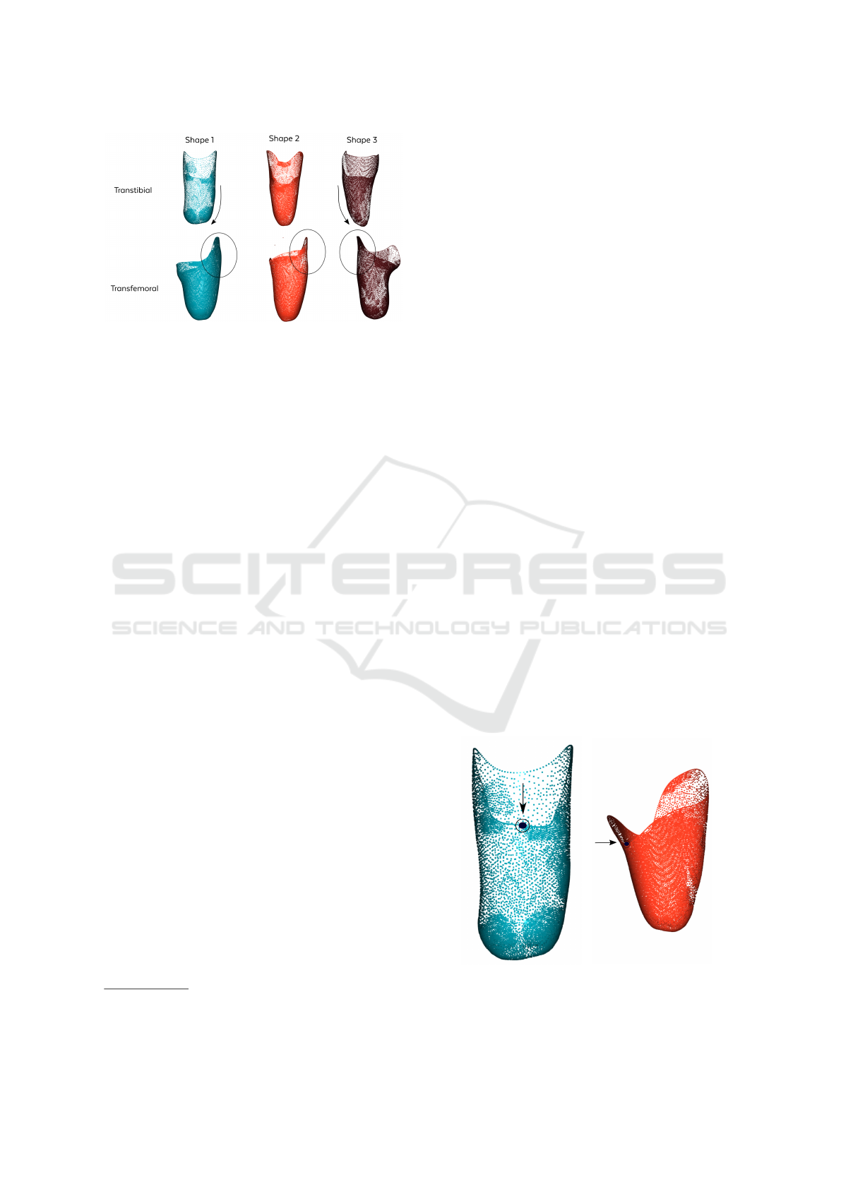
Figure 1: Transtibial and transfemoral sockets from the
dataset, in posterior views, with medial leaning and lateral
support highlighted.
digitizes the interior surface of sockets
1
. These scans
were acquired in clinical settings with the use of the
data for research purposes authorized. Scans have no
associated patient information other than the type of
amputation and the leg. For each scan, multiple mea-
sures were taken to characterize the socket, namely its
full height (MaxH) and the maximum height at which
the perimeter still corresponds to a full circle (MinH),
and the socket perimeters at MinH, at mid-height and
at the bottom (HP, MP and BP, respectively).
Some examples of the dataset can be seen in Fig-
ure 1. Anatomical variations such as length of the
residual limb or musculature (reflected in a more con-
ical shape) can be seen, along with more distinctive
features such as the medial leaning of TT sockets. A
total of 30 TT and 21 TF examples were collected.
The analysis of their characteristics is summarized in
Table 1.
3.2 Point Cloud Registration
3.2.1 Alignment
Due to the inherent differences between shapes of TT
and TF sockets, two separate but analogous proce-
dures were followed for registration. For both types
of sockets, the final registration result was determined
to be a point cloud with as many points as the smallest
point cloud in the dataset (4,731 for TT and 11,487 for
TF). The acquisition system guarantees that the ac-
quired shapes are all under the same metric referential
and that the vertical axes of the sockets are aligned.
Therefore, the alignment problem is simplified to a
two-dimensional rotation and a translation.
The translation problem was solved by overlap-
ping the centroids of each socket with the origin of
the coordinate system.
1
INSIGHT™ Scanner: https://www.adapttech.eu/
insight#knowinsight
The rotation required an additional pre-processing
step: the mirroring of shapes pertaining to the left
leg along a radial plane, to harmonize differences be-
tween left and right leg. Then, to find the optimal 2D
rotation matrix to align the shapes, a landmark present
across all shapes (based on domain knowledge) was
chosen. The optimal rotation was finally defined as
that which brings these landmarks into overlapping
positions. For TT sockets, the landmark chosen was
the center of the posterior proximal support, as seen in
Figure 2a. For TF sockets, the landmark was the cen-
ter of the medial proximal border, as seen on Figure
2b.
A semi-automatic method was employed to de-
tect these landmarks using the measurements taken
for each instance of the dataset.
To overlap the landmarks, a socket from the
dataset was randomly chosen as the target and all
other point clouds were aligned relative to it.
3.2.2 Correspondence
Two different methods were tested to establish point-
to-point correspondence: local feature similarity us-
ing Fast Point Feature Histograms and a custom
heuristic henceforth referred to as Selective Sam-
pling.
Fast Point Feature Histograms. (FPFH) are local
descriptors which have been used in state-of-the-art
applications for point cloud registration. This descrip-
tor relies on the angular relationships between the nor-
mals of a given point and its neighbours to compute
descriptive histograms. From these descriptors, cor-
respondence can be established between points which
have the most similar features by computing the his-
tograms’ distances (Rusu et al., 2009).
Selective Sampling: is based on a registration tech-
(a) Posterior view of TT
socket.
(b) Anterior-Medial
view of TF socket.
Figure 2: Landmarks chosen for TT and TF sockets.
VISAPP 2021 - 16th International Conference on Computer Vision Theory and Applications
530

Figure 3: Two sockets registered through Selective Sam-
pling. For a given height percentage h, a socket’s circular
profile has N points separated by an angle α.
nique often used in statistical shape models, which
is parametrization by sampling evenly spaced points
across a contour. Using domain knowledge and a
more intuitive notion of correspondence, a similar ap-
proach which performs a selective sampling on the
point clouds was designed. Two corresponding points
can be thought of as points which are in the same
relative position on two different sockets. Since the
sockets are approximately paraboloids, this position
can be defined by two values: the angle ω relative to
a known vector and a percentage h of the height in
two regions: above the landmark, and below the land-
mark. These two regions assure that the posterior and
anterior support will always correspond across sock-
ets, even if the lateral support’s height differs between
them.
The reference vector used to define the angle was
the the origin-landmark vector OL used for alignment
(where origin corresponds to the center of the circum-
ference at the same z as the landmark). This vector is
translated to a given height percentage h, OL
h
and ro-
tated around the z-axis in N intervals of α degrees.
Rotating OL
h
around the vertical z-axis by this angle
creates a set P
t
of evenly spaced target coordinates in
the shape of a circular profile:
P
t
(h, ω) = OL
h
× R
z
(i × α) (1)
where i ∈ [0, ... , N] and R
z
is the rotation matrix
around z. Each point P
t
(h, ω) in P
t
is then matched
to its closest neighbour in the point cloud A which
has not yet been matched (to ensure a one-to-one cor-
respondence):
P(h, ω) = arg min
p∈A
(||p − P
t
(h, ω)||) (2)
The final registration result is then controlled by
two parameters: N, the number of points in each
circular profile, and K the number of profiles which
should be sampled across the socket height. Figure
3 shows a schematic representation of the selective
sampling process.
3.3 Model Building
With properly aligned and registered socket shapes,
a statistical shape model F can be built from the
dataset. PCA was performed for each separate type
of socket, since the base designs of TT and TF vary
considerably. To perform PCA on a registered train-
ing set, Singular Value Decomposition is applied to
the shapes F − F, where F is the mean of the aligned
shapes. The resulting matrix is a matrix P of eigen-
vectors, as well as their corresponding eigenvalues λ.
Any valid shape set can then be defined as:
F = F +
M
∑
m=1
PC
m
b
m
(3)
where M is the number of eigenvectors in the model
(subspace dimension), b
m
are scalar weights and PC
m
are the principal components. To assure plausible
variation, b
m
has to be limited. Typical values to con-
strain this variation are [−3λ
m
, 3λ
m
]. For both TT
and TF sockets, two different models were built, us-
ing the shapes registered through Selective Sampling
and FPFH.
3.4 Evaluation
Generalization reflects the ability of a model to de-
scribe instances of the object that have not been
seen during model building. If a model is overfit-
ted, then its ability to generalize when faced with a
new example will be very low. Generalization can be
measured with a leave-one-out methodology (Davies
et al., 2010).
Specificity is a measure of the similarity between
generated shapes and the ones present in the training
set. It is quantitatively defined by generating a new
population of instances and averaging the distance be-
tween a new generated shape and the closest shape to
it in the training set. The new population of instances
should be created with weights that assure plausible
shapes. This, combined with generalization, evalu-
ates both the generative and reconstructive abilities of
the model.
A visual expert evaluation was also performed by
determining the individual meaning of each principal
component (PC) captured by the model and and at-
tributing it an anatomical interpretation (when such
interpretation existed in the prosthetics domain).
Generalization and specificity are two com-
mon approach-independent metrics used in the field
(Davies et al., 2010). Due to the reduced size of the
dataset, no explicit training/testing set division was
done. This omission is counterweighted by the evalu-
ation of generalization - a proxy metric of overfitting.
Embedding Anatomical Characteristics in 3D Models of Lower-limb Sockets through Statistical Shape Modelling
531
Table 2: Weight factors of each visually interpretable principal component, as validated by ortoprosthetists.
PC1 PC2 PC3 PC4 PC5 PC6
Min Max Min Max Min Max Min Max Min Max Min Max
TT -30 30 - - -20 30 -5 15 - - -15 15
TF -30 30 -30 30 -15 10 -15 30 -12 12 -10 15
Figure 4: Generalization comparison between transtibial
models registered through Selective Sampling and FPFH.
4 RESULTS
Results on generalization and specificity are pre-
sented for models based on point clouds registered
through Selective Sampling and FPFH. This allows
for a comparison between the accuracy of both meth-
ods, since a better registration will lead to a better
model. Specificity and generalization were computed
using as distance measure a normalized (by the num-
ber of points in question) Mean Absolute Distance
(mean of the absolute distance between correspond-
ing points, MAD).
Regarding expert evaluation, orthoprosthetists
contributed to results by defining weight limits that
assure the generation of plausible shapes (Table 2).
These weights were applied for the generation of
new shapes, both for specificity calculation and for
the visualization of PC effects on the average shape
(using Equation (3)). For components with no visual
interpretation, the weights used were [−3λ
m
, 3λ
m
],
as common in the literature.
Results subject to comparison were not found in
the authors’ literature review.
4.1 Transtibial Statistical Shape Model
4.1.1 Model Performance
By analysing the cumulative variance of the models,
it is possible to determine how many PCs are required
to obtain a descriptive model. To describe 95% of
the variance in the training dataset, the Selective Sam-
Figure 5: Specificity comparison between transtibial mod-
els registered through Selective Sampling and FPFH.
pling model requires 6 PCs, while the FPFH one re-
quires 22.
As shown in Figure 4, the model built from Selec-
tive Sampling registration has a lower reconstruction
error, meaning better generalization. As expected,
generalization improves with the number of principal
components used for reconstruction. With 6 PCs, Se-
lective Sampling produces a reconstruction error of
6.8 ± 1.8 mm, while FPFH at 22 PCs surpasses this
error, with 21.6 ± 2.4 mm.
Specificity, which represents the similarity be-
tween the generated shapes and the ones present in
the training set, is again superior using Selective Sam-
pling (Figure 5), with an error of 9.7 ± 0.6 mm.
Specificity is a crucial parameter in this work, given
that one of the proposed applications is the creation
of plausible shapes.
Since the models registered through Selective
Sampling outperformed FPFH in all metrics, this
model was chosen for the subsequent analyses.
4.1.2 Principal Component Analysis
In partnership with orthoprosthetists, it was possible
to derive anatomical interpretations of the variance
components captured by the model. PCs in which no
relevant anatomical or design information was identi-
fied were omitted.
The first PC, which represents around 70% of the
total variance, is related to the length of the residual
limb, as can be seen in Figure 6. This is a natural
variation, since the level of amputation is highly vari-
able, depending on the patient’s anatomy and injury
degree.
VISAPP 2021 - 16th International Conference on Computer Vision Theory and Applications
532
Figure 6: Representation of the principal components PC1
(residual limb length), PC3 (residual limb volume), PC4
(patellar coverage) and PC6 (medial leaning) with eigen-
values (λ), over the average transtibial shape (µ) and weight
factors (WF) from Table 2 (posterior view).
The third PC, accounting for 5% of variance, cor-
responds to the circular profile variation along the lon-
gitudinal axis, distinguishing between more conical
or cylindrical sockets. This is related to the muscula-
ture of the residual limb, which varies between sub-
jects and also in time, since residual limbs are prone
to atrophy and volume variations. Figure 6 shows
this effect: the leftmost sockets exhibits perimeter re-
duction along its longitudinal axis, creating a conical
shape, unlike the rightmost one, where the perimeter
varies a lot less.
The fourth PC, responsible for 2.5% of the vari-
ance, is related to the level of coverage of the kneecap.
Different designs can cover more or less of the knee
structure, which is reflected in Figure 6. For instance,
the leftmost socket, with higher lateral and medial
walls and more patellar coverage, has a design evok-
ing a suprapatellar patellar-tendon bearing socket (Pa-
tern
`
o et al., 2018).
The sixth PC, representing 1% of the variance,
represents a lateral-medial leaning in the socket (Fig-
ure 6), along with a narrowing of the distal end. This
is frequently observed and depends on several factors:
the level of amputation and the natural muscular pro-
file and bone structure of the lower limb.
Figure 7: Generalization comparison between transfemoral
models registered through Selective Sampling and FPFH.
Figure 8: Specificity comparison between transfemoral
models registered through Selective Sampling and FPFH.
4.2 Transfemoral Statistical Shape
Model
4.2.1 Model Performance
A similar analysis to the one performed for the TT
model can be done for the TF model. To describe 95%
of the variance in the training dataset, the Selective
Sampling model requires 11 PCs, while the FPFH one
requires 16.
For a model with 11 PC, representing 95% of
the variation in the training set, the generalization
through Selective Sampling is 10.5 ± 1.6 mm, mean-
ing an unseen shape would be, on average, recon-
structed with this error. As shown in Figure 7, the Se-
lective Sampling model again outperformed the FPFH
registration. The generalization ability for this model
is inferior to the one found for TT sockets.
Finally, the specificity of the TF model was also
inferior to the TT one, with an error of 9.8 ± 0.2 mm
for the Selective Sampling model (Figure 8).
Similarly to the TT case, the model registered
Embedding Anatomical Characteristics in 3D Models of Lower-limb Sockets through Statistical Shape Modelling
533
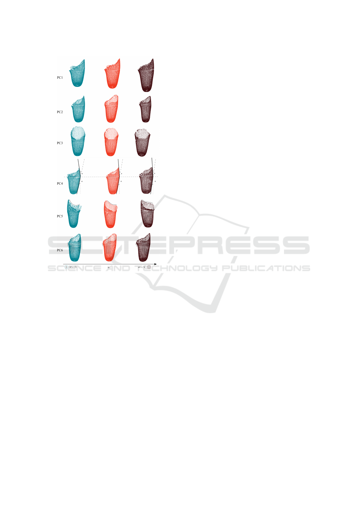
Figure 9: Representation of the influence of principal com-
ponents: PC1 (residual limb length), PC2 (residual limb
volume), PC3 (height of the lateral support), PC4 (adduc-
tion angle), PC5 (posterior proximal contour) and PC6 (is-
chial support) with eigenvalues (λ), over the average trans-
femoral shape (µ), with weight factors (WF) from Table 2.
PC1, PC2, PC4 and PC6 are shown in a posterior view, PC3
in a medial view and PC5 in an anterior view.
through Selective Sampling outperformed FPFH in all
metrics, and was, therefore, the one chosen for subse-
quent analyses.
4.2.2 Principal Component Analysis
The most significant variation in the TF shapes is
again relative to the length of the residual limb, rep-
resenting 64% of the variance (Figure 9).
The second PC is related to the circular profiles
along the longitudinal axis, responsible for 12% of
variance. A more conical stump can be seen on the
rightmost socket of Figure 9, while the leftmost one
would be appropriate for a more cylindrical stump.
This profile is dependent on the amputee’s muscula-
ture and time after amputation, since the muscles are
subject to atrophy and volume reductions.
The third PC, which accounts for 5% of variance,
represents the height of the lateral support. In Figure
9, the leftmost point cloud has a higher lateral support,
which decreases in the shapes to its right.
PC number four is related with the adduction an-
gle of the femur and the ilio-femoral angle, two im-
portant measurements taken during the fitting process,
and represents 4% of variance. The first is defined be-
tween a longitudinal axis and the femur while in max-
imal adduction and is typically larger for women. The
second is defined between the femur line and the lat-
eral support. Figure 9 shows that, from left to right,
these angles decrease.
The fifth PC varies the shape of the posterior prox-
imal contour of the socket. In Figure 9, it is possible
to see that the valley between the lateral and ischial
support is more pronounced in the leftmost shape.
This contour has an important effect in the aesthetic
effect of the socket, as well as in comfort while sit-
ting.
The sixth PC, which accounts for 2.5% of vari-
ance, is related to the prominence of the ischial seat.
In Figure 9 (left of the top contour), it is possible to
see that, from left to right, this support becomes wider
and more pronounced.
5 DISCUSSION & CONCLUSIONS
By observing the features captured by the models, it
is possible to conclude that they represent important
anatomical variations in socket design - such as length
and profile, in coherence with (Steer et al., 2020), but
also subtler design characteristics. Given this, these
models can be useful for generating new shapes with
specific characteristics by manipulating the influence
of their respective PCs. Additionally, the model’s
good generalization abilities allow it, for instance, to
be used to reconstruct new 3D scans in socket acqui-
sition systems, which may minimize acquisition arti-
facts.
The analysis performed showed the TT model out-
performed the TF in all metrics. This can be due to
a larger variation across base TF designs, which, in
turn, can lead to a poorer registration process, or sim-
ply due to the lower number of samples used to build
the model.
Two import aspects limit our work. Firstly, the
high dependence on the registration process, which
heavily impacts the input of the PCA model and,
therefore, the accuracy of the results. To improve re-
sults and reduce that dependency, other more robust
local descriptors could be tested. Secondly, the in-
VISAPP 2021 - 16th International Conference on Computer Vision Theory and Applications
534

ability to directly compare with other authors. This
stems from the lack of relevant work in this field (as
far as we were able to ascert) and the lack of reference
datasets for the task. Towards mitigating the latter, we
are making some example data available in Section 6.
Nevertheless, this work shows that mathemati-
cally representing socket point cloud data through sta-
tistical shape models encodes biomechanically rele-
vant information, allowing a range of potential ap-
plications with clinical interest like the generation of
new plausible socket shapes (to support data-intensive
learning workflows) or the automatic rotation of sock-
ets’ point clouds into relevant anatomical planes (for
improved user experience in CAD/CAM software).
6 CONTRIBUTIONS
Some examples of TT and TF sockets shapes gener-
ated with the SSM are available on a GitHub reposi-
tory: https://github.com/adapttech-ltd/SocketSSM.
REFERENCES
Castellani, U. and Bartoli, A. (2014). 3D shape regis-
tration. In 3D Imaging, Analysis and Applications,
volume 9781447140, pages 221–264. Springer-Verlag
London Ltd.
Cha, J., Farhangi, M. M., Dunlap, N., and Amini, A. A.
(2018). Segmentation and tracking of lung nodules
via graph-cuts incorporating shape prior and motion
from 4D CT. Medical Physics, 45(1):297–306.
Cootes, T. F., Taylor, C. J., Cooper, D. H., and Graham, J.
(1992). Active Shape Models-Their Training and Ap-
plication. Computer Vision and Image Understanding,
61(1):38–59.
Davies, R., Twining, C., Cootes, T., and Taylor, C. (2010).
Building 3-D Statistical Shape Models by Direct Op-
timization. IEEE Transactions on Medical Imaging,
29(4):961–981.
Huang, H., Brenner, C., and Sester, M. (2013). A generative
statistical approach to automatic 3D building roof re-
construction from laser scanning data. ISPRS Journal
of Photogrammetry and Remote Sensing, 79:29–43.
Karakoc¸, M., Batmaz, I., Sariyildiz, M. A., Yazmalar, L.,
Aydin, A., and Em, S. (2017). Sockets Manufactured
by CAD CAM Method Have Positive Effects on the
Quality of Life of Patients With Transtibial Amputa-
tion. American Journal of Physical Medicine & Reha-
bilitation, 96(8):578–581.
Lindner, C. (2017). Automated Image Interpretation Us-
ing Statistical Shape Models. In Statistical Shape and
Deformation Analysis: Methods, Implementation and
Applications, pages 3–32. Elsevier Inc.
Mehmood, W., Abd Razak, N. A., Lau, M. S., Chung, T. Y.,
Gholizadeh, H., and Abu Osman, N. A. (2019). Com-
parative study of the circumferential and volumet-
ric analysis between conventional casting and three-
dimensional scanning methods for transtibial socket:
A preliminary study. Proceedings of the Institution of
Mechanical Engineers, Part H: Journal of Engineer-
ing in Medicine, 233(2):181–192.
Patern
`
o, L., Ibrahimi, M., Gruppioni, E., Menciassi, A.,
and Ricotti, L. (2018). Sockets for Limb Prostheses:
A Review ofExisting Technologies and Open Chal-
lenges. IEEE Transactions on Biomedical Engineer-
ing, 65(9):1996–2010.
Pedregosa, F., Varoquaux, G., Gramfort, A., Michel, V.,
Thirion, B., Grisel, O., Blondel, M., Prettenhofer,
P., Weiss, R., Dubourg, V., Vanderplas, J., Passos,
A., Cournapeau, D., Brucher, M., Perrot, M., and
Duchesnay, E. (2011). Scikit-learn: Machine learning
in Python. Journal of Machine Learning Research,
12:2825–2830.
Rusu, R. B., Blodow, N., and Beetz, M. (2009). Fast point
feature histograms (fpfh) for 3d registration. In 2009
IEEE International Conference on Robotics and Au-
tomation, pages 3212–3217.
Steer, J. W., Worsley, P. R., Browne, M., and Dickinson,
A. S. (2020). Predictive prosthetic socket design: part
1-population-based evaluation of transtibial prosthetic
sockets by FEA-driven surrogate modelling. Biomech
Model Mechanobiol, 19(4):1331–1346.
Van Der Walt, S., Colbert, S. C., and Varoquaux, G. (2011).
The numpy array: a structure for efficient numerical
computation. Computing in Science & Engineering,
13(2):22.
Varma, P., Stineman, M. G., and Dillingham, T. R. (2014).
Epidemiology of limb loss. Physical Medicine and
Rehabilitation Clinics of North America, 25(1):1–8.
Wurdeman, S. R., Stevens, P. M., and Campbell, J. H.
(2018). Mobility Analysis of AmpuTees II: Comor-
bidities and Mobility in Lower Limb Prosthesis Users.
American Journal of Physical Medicine and Rehabil-
itation, 97(11):782–788.
Yang, F., Metaxas, D., Wang, J., Shechtman, E., and Bour-
dev, L. (2011). Expression Flow for 3D-Aware Face
Component Transfer. ACM Transactions on Graphics,
30(4):1–10.
Yang, J., Cao, Z., and Zhang, Q. (2016). A fast and robust
local descriptor for 3D point cloud registration. Infor-
mation Sciences, 346-347:163–179.
Zhou, Q.-Y., Park, J., and Koltun, V. (2018). Open3D:
A modern library for 3D data processing.
arXiv:1801.09847.
Embedding Anatomical Characteristics in 3D Models of Lower-limb Sockets through Statistical Shape Modelling
535
