S*ReLU: Learning Piecewise Linear Activation Functions
via Particle Swarm Optimization
Mina Basirat
1 a
and Peter M. Roth
1,2 b
1
Institute of Computer Graphics and Vision, Graz University of Technology, Austria
2
Data Science in Earth Observation, Technical University of Munich, Germany
Keywords:
Visual Categorization, Activation Functions, Particle Swarm Optimization.
Abstract:
Recently, it was shown that using a properly parametrized Leaky ReLU (LReLU) as activation function yields
significantly better results for a variety of image classification tasks. However, such methods are not feasible
in practice. Either the only parameter (i.e., the slope of the negative part) needs to be set manually (L*ReLU),
or the approach is vulnerable due to the gradient-based optimization and, thus, highly dependent on a proper
initialization (PReLU). In this paper, we exploit the benefits of piecewise linear functions, avoiding these
problems. To this end, we propose a fully automatic approach to estimate the slope parameter for LReLU from
the data. We realize this via Stochastic Optimization, namely Particle Swarm Optimization (PSO): S*ReLU. In
this way, we can show that, compared to widely-used activation functions (including PReLU), we can obtain
better results on seven different benchmark datasets, however, also drastically reducing the computational
effort.
1 INTRODUCTION
In the recent years, there has been a large scien-
tific interest in manually designing (Klambauer et al.,
2017; Clevert et al., 2016; Elfwing et al., 2018; Glo-
rot et al., 2011; Gulcehre et al., 2016)) and learn-
ing (Ramachandran et al., 2018; Basirat and Roth,
2019; Hayou et al., 2018; Li et al., 2018) new activa-
tion functions (AFs). Even though these works could
show that using more sophisticated non-linearities is
beneficial in terms of convergency and training stabil-
ity, for many tasks—including image classification—
those are not reflected by the final performance. The
reported improvements, if any, are often only very
small. Thus, for many practical applications, ReLU is
still used as non-linearity. This, however, is only true
if the data is well separable. In contrast, if we have to
deal with hard-to-distinguish classes, and even subtle
differences are of relevance, using more sophisticated
activation functions gives significantly better results
(Basirat and Roth, 2020). In particular, using a prop-
erly initialized Leaky ReLU (L*ReLU) enforces the
class separability and, finally, gives significantly bet-
ter results.
a
https://orcid.org/0000-0001-5902-3045
b
https://orcid.org/0000-0001-9566-1298
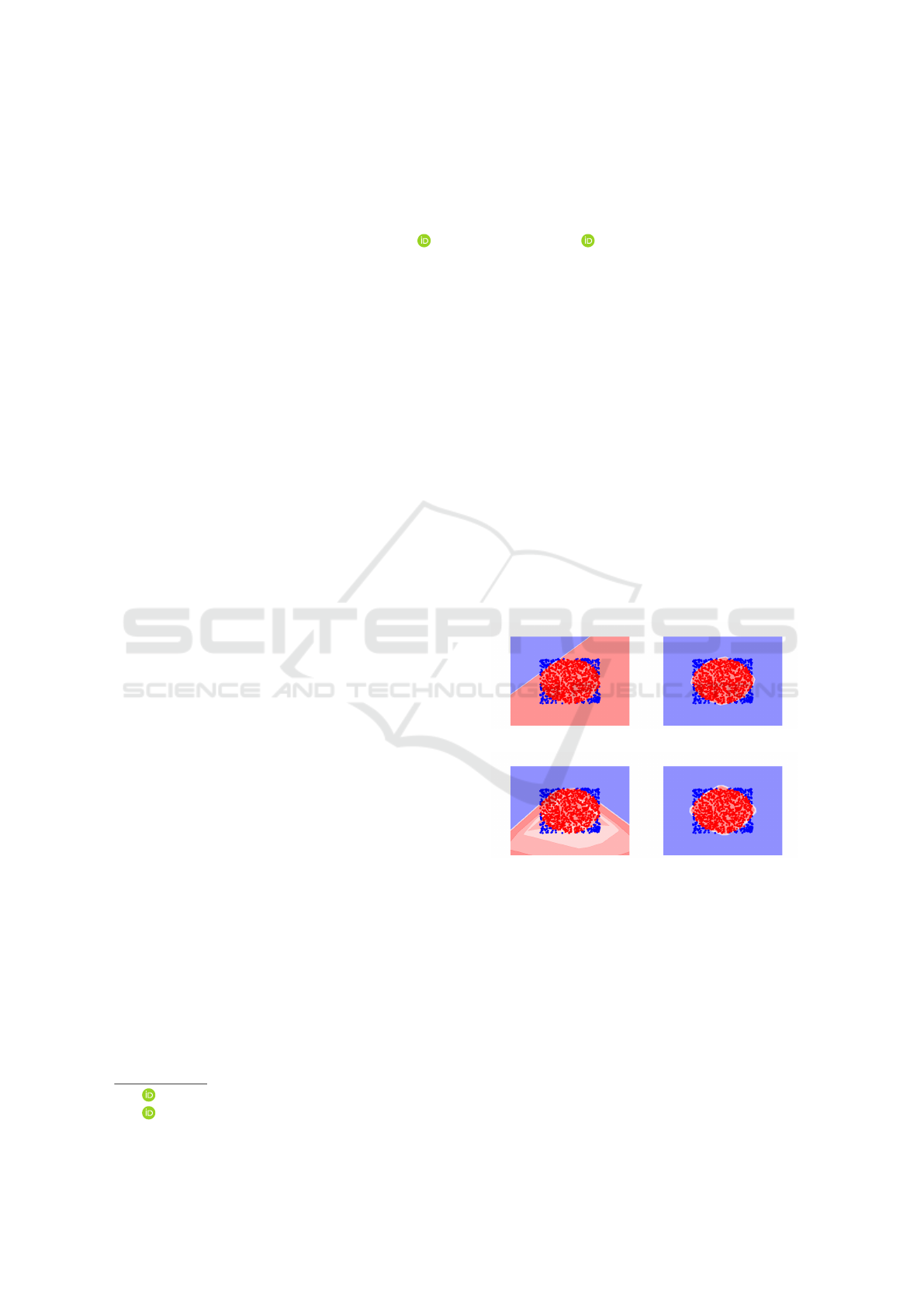
(a) ReLU. (b) L*ReLU.
(c) PReLU. (d) S*ReLU (proposed).
Figure 1: Nonlinear classification problem solved using
different activation functions: (a) ReLU, (b) L*ReLU, (c)
PReLU, and (d) S*ReLU (proposed).
To illustrate this, in Fig. 1, we show the decision
boundaries for a simple nonlinear two-class classifi-
cation problem, defined as separating the red points
within a circle from the blue points outside the cir-
cle. Therefore, we apply a shallow fully connected
network with three layers (2,4,2), using different acti-
vation functions. From Fig. 1(a) we can see that using
ReLU even this simple problem cannot be solved. In
contrast, Fig. 1(b) shows that L*ReLU using a prop-
Basirat, M. and Roth, P.
S*ReLU: Learning Piecewise Linear Activation Functions via Particle Swarm Optimization.
DOI: 10.5220/0010338506450652
In Proceedings of the 16th International Joint Conference on Computer Vision, Imaging and Computer Graphics Theory and Applications (VISIGRAPP 2021) - Volume 5: VISAPP, pages
645-652
ISBN: 978-989-758-488-6
Copyright
c
2021 by SCITEPRESS – Science and Technology Publications, Lda. All rights reserved
645

erly set negative slope allows for perfectly separating
the two classes. However, in this case, the optimal
parameter needs to be searched by a time-consuming
grid-search, which is not feasible in practice.
To reduce the effort and the computational costs,
an automatic approach preserving the positive proper-
ties of linear piecewise activation functions would be
desirable. For instance, Parametric ReLU (PReLU)
(He et al., 2015) learns the slope parameter from the
training data. However, the approach is based on
gradient-based optimization. Thus, the optimization
likely gets stuck into a local optimum, and the suc-
cess of the approach strongly depends on the initial-
ization. This is illustrated in Fig. 1(c), showing that,
in the expected case, the classification problem cannot
be solved properly.
To summarize, it is neither desirable to estimate
the necessary parameter manually (L*ReLU), nor to
rely on a gradient-based approach, which highly de-
pends on a proper initialization (PReLU). To avoid
both shortcomings, we propose to automatically learn
the slope parameter from the data, adopting ideas
from Stochastic Optimization (Spall, 2003). In con-
trast to gradient-based approaches, we avoid getting
stuck into local optima, and can ensure a globally op-
timal solution. Thus, as can be seen in Fig. 1(d), we
can estimate the decision boundary very well, even
though no prior knowledge was used. In favor of
other stochastic optimization methods, we finally se-
lected Particle Swarm Optimization (PSO) (Eberhart
and Kennedy, 1995) due to its simplicity and effi-
ciency.
The experimental results on seven different
datasets show that, in this way, the optimal slope can
be estimated, even though no prior knowledge was
used, and that even the accuracy level of L*ReLU can
be matched. In addition, we compare our results with
those obtained by well-known and widely-used acti-
vation functions as well as to PReLU, which also es-
timates the slopes automatically from the data.
Thus, the main contributions of this paper can be
summarized as follows:
• We introduce a Particle Swarm Optimization
(PSO) based approach to automatically estimate
the optimal slope of the negative part of Leaky
ReLU (LReLU). Thus, also building on the ideas
of L*ReLU, we would like to refer to it as
S*ReLU.
• We demonstrate that our fully automatic approach
finally matches the accuracy level of L*ReLU,
which uses the manually-set optimal parameter
and, thus, yields the best possible solution (esti-
mated via a thorough parameter search).
2 RELATED WORK
In the following, we, first, give a summary of fixed
(Sec. 2.1) and learned (Sec. 2.2) activation functions.
Then, we revise Leaky ReLU in more detail (Sec. 2.3).
Finally, we give a short introduction to metaheuristic
stochastic optimization (Sec. 2.4).
2.1 Fixed Activation Functions
Inspired by simple thresholding functions, in the first
place, squashing functions such as Sigmoid and Tanh
(Hornik, 1991) were of interest. In particular, as they
are continuous, bounded, and monotonically increas-
ing, they fulfill the required properties of the univer-
sal approximation theorem (Hornik, 1991), making
them a valid choice when learning continuous non-
linear functions. However, such functions often suf-
fer from the vanishing gradient problem (Hochreiter,
1998), which is, in particular, a problem when net-
works are getting deeper.
To overcome this problem, Rectified Linear Units
(ReLU) (Nair and Hinton, 2010) have been intro-
duced. As the derivative of any positive input is one,
the gradient cannot vanish, whereas all negative val-
ues are mapped to zero. On the one hand, this makes
ReLU easily and efficiently applicable; on the other
hand, we are facing two main problems: (a) There
is no information flow for negative values, which is
known as dying ReLU. (b) The statistical mean of the
activation values is larger than zero, leading to a bias
shift in successive layers.
Both shortcomings can be alleviated by using Ex-
ponential Linear Unit (ELU) (Clevert et al., 2016).
By pushing the mean activation value towards zero,
ELU is more robust to noise and eliminates the bias
shift in the succeeding layers. This idea was later
extended by introducing a self-normalizing network:
Scaled Exponential Linear Unit (SELU) (Klambauer
et al., 2017). In this way, convergence towards a nor-
mal distribution with zero mean and unit variance can
be ensured.
2.2 Learned Activation Functions
More efficient activation functions can be obtained by
learning the parameters from the data. In this way,
Parametric ELU (Trottier et al., 2017) overcomes the
vanishing gradient problem and allows for controlling
the bias shift. More complex functions (also non-
convex ones) can be learned using Multiple Paramet-
ric Exponential Linear Units (Li et al., 2018). In this
way, better convergence properties can be ensured, fi-
nally, leading to a better classification performance.
VISAPP 2021 - 16th International Conference on Computer Vision Theory and Applications
646

Similar results can also be achieved by adopting ideas
from reinforcement learning (Ramachandran et al.,
2018) and genetic programming (Basirat and Roth,
2019) by exploring complex search spaces, allow-
ing to construct new, more complex AFs. In this
way, Swish (Ramachandran et al., 2018), a combina-
tion of a squashing and a linear function, was found,
which has been demonstrated to work very well for
many problems. As an extension, Parametric Swish
(PSwish) additionally allows to train a scaling param-
eter. Similar functions, also yielding slightly better re-
sults in the same application domains, were found by
(Basirat and Roth, 2019). Recently, a theoretic jus-
tification for these results has been given in (Hayou
et al., 2018), demonstrating that Swish-like functions
propagate information better than ReLU.
Even though competitive results have been shown
for many problems, the beneficial theoretical proper-
ties did not allow to (significantly) outperform neural
networks using ReLU. Thus, for most applications,
ReLU is used as nonlinearity, and other activation
functions are not considered at all.
2.3 Leaky ReLU
Nevertheless, it was shown that using Leaky ReLU
(LReLU) (Maas et al., 2013), just introducing a small
slope (α = 0.01) for the negative part of ReLU, gives
better results for many tasks. Even though we can
overcome the dying-ReLU-problem, we are still suf-
fering from the bias shift. In this way, Random-
ized Leaky Rectified Linear Unit (RReLU) (Xu et al.,
2015) sets the slope for the negative part randomly.
Recently, it has been shown that not only using a
non-zero negative part is essential, but that also the
slope of the negative part is of importance. In par-
ticular, the goal of L*ReLU (Basirat and Roth, 2020)
was to demonstrate two points: First, piecewise linear
activation functions can deal with more complex data
very well, i.e., if the data is not well separable. This
is, in particular, the case when classes are very simi-
lar and small subtle differences need to be modeled.
Therefore, also the absence of features needs to be
covered. To this end, an activation function needs to
be uniform-continuous and strictly increasing, which
can be ensured by a probably initialized LReLU. Sec-
ond, the optimal slope is highly data-dependent and
related to the Lipschitz constant (c.f., (Sokoli
´
c et al.,
2017; Anil et al., 2019; Tsuzuku et al., 2018)). Thus,
for different tasks also different parameters for the
negative slope are needed. Even though these are in-
teresting insights, the slope for L*ReLU needs to be
set manually, which is infeasible in practice.
Parametric ReLU (PReLU) (He et al., 2015) over-
comes this problem by learning the slopes for the neg-
ative part based on the training data. Moreover, there
are two main differences to L*ReLU: (a) a separate
activation function is learned for each layer, and (b)
the activation functions are not kept fixed but are up-
dated during neural network training. Even though
this sounds reasonable, the main drawback of PReLU
is—building on a gradient-based optimization—that
the solver often gets stuck into a local optimum, mak-
ing the approach very sensitive to a proper initializa-
tion. To allow to generate complex functions, SReLU
(Jin et al., 2016) is defined via three piecewise linear
functions finally forming a crude S shape.
Overall, neither manually setting the slope param-
eter nor a high sensitivity to the initialization are de-
sirable in practice. Thus, in the following, we intro-
duce an approach for learning piecewise linear func-
tions from the data, overcoming the problems dis-
cussed above by building on ideas from metaheuristic
stochastic optimization.
2.4 Metaheuristic Stochastic
Optimizations
During the last decades, various metaheuristic
stochastic optimization approaches (Osman and La-
porte, 1996) such as Evolutionary Algorithms (EA)
(e.g., (Koza et al., 1999; Schwefel, 1987; Goldberg,
1989; Holland, 1992)) or Particle Swarm Optimiza-
tion (PSO) (Eberhart and Kennedy, 1995) have been
introduced. The key idea of such approaches is that
a population of candidate solutions competes and/or
collaborates to find the optimal solution through eval-
uating the fitness of each candidate solution. Then,
each candidate solution is tweaked over several iter-
ations in the direction of the fittest solution. Indeed,
Evolutionary Algorithms (EA), including Genetic Al-
gorithms (GA) (Goldberg, 1989; Holland, 1992), Ge-
netic Programming (GP) (Koza et al., 1999), and Evo-
lution Strategies (ES) (Schwefel, 1987), are inspired
from biology. In contrast, PSO is a swarm intelli-
gence algorithm inspired by the social behaviors of
a swarm. Therefore, candidate solutions are referred
to as a swarm of particles, not as a population of indi-
viduals. In contrast to EAs, PSO does not re-sample
particles to generate new ones. PSO has been widely
used for hyper-parameter tuning and designing the
topology of deep neural networks (Sinha et al., 2018;
Lorenzo et al., 2017; Wang et al., 2018). Due to its
simplicity and the ability also to deal with rather com-
plex problems, for our problem, we finally decided to
build on PSO in favor of other metaheuristic stochas-
tic optimization approaches.
S*ReLU: Learning Piecewise Linear Activation Functions via Particle Swarm Optimization
647

3 LEARNING PIECEWISE
LINEAR ACTIVATION
FUNCTIONS
In the following, in Sec. 3.1, we first review the main
concepts and motivation of piecewise linear activa-
tion functions, in particular of Rectified Linear Unit
(ReLU) and Leaky Rectified Linear Unit (LReLU).
Then, in Sec. 3.2, we introduce our new, more robust
automatic approach to estimate the optimal slope for
the negative part of LReLU.
3.1 Piecewise Linear Activation
Functions
Piecewise functions, in general, are defined via dif-
ferent functions for different parts of the domain. In
our case, we are interested in piecewise linear func-
tion f (x) defined for the negative, f (x ≤ 0), and the
positive, f (x > 0), domain of R. The most promi-
nent function of this family is Rectified Linear Unit
(ReLU) defined as
f (x) = max(x, 0). (1)
In practice, for most applications, including im-
age classification, ReLU is used due to its simplicity
and efficiency. Moreover, for a wide range of appli-
cations, good results can be obtained. However, due
to the constantly zero negative part, we are suffering
from the dying ReLU problem and a bias shift in sub-
sequent layers. To this end, it has been shown that in-
troducing a small negative slope (i.e., α = 0.01) gives
better results for many applications:
f (x) = max(x, 0) + min(αx, 0), (2)
where α ≥ 0 defines the slope of the linear function
for the negative part. The function f (x) defined in
Eq. (2) is referred to as Leaky ReLU (LReLU). As can
be seen from Fig. 2, the main difference compared
to ReLU is that not all negative values are mapped
to zero but are mapped using a linear function with a
small slope α.
−4 −2 2
−1
1
2
3
−4 −2 2
−1
1
2
3
(a) f (x) = ReLU. (b) f (x) = LReLU.
Figure 2: Piecewise linear functions: (a) ReLU and
(b) Leaky ReLU (LReLU), consisting of two linear parts:
f (x ≤ 0) and f (x > 0).
More recently, in (Basirat and Roth, 2020) it has
been demonstrated that not only using a non-zero neg-
ative part is of importance, but that also the selected
slope is of relevance. Moreover, it has been revealed
that the optimal slope is data-dependent. In other
words, for different tasks a different parametrization
is necessary. In general, as long as the data is well-
separable in the latent space, the choice of the activa-
tion function is not critical. This is also illustrated
in Table 3, where it can be seen that for different
choices of activation functions very similar results are
obtained for the CIFAR-datasets.
If this is not ensured, it has been shown (Basirat
and Roth, 2020; Clevert et al., 2016) that also
modeling the absence of features is of importance,
which can be achieved via using strictly monotoni-
cally increasing non-linear functions that are uniform-
continuous. In practice, this means that the negative
values should neither be mapped to zero nor satu-
rating, and that similar inputs should produce simi-
lar outputs. Both properties are fulfilled by LReLU,
where, additionally, also the desirable properties of
ReLU are inherited.
Even though this is an important and interesting
insight, it is not convenient to set the necessary pa-
rameter manually. To overcome this problem, PReLU
(He et al., 2015) can be used, which automatically
estimates the optimal slopes (i.e., separately for each
layer) from the data. However, as also can be seen
from Tables 3 and 4, the success of the approach is
highly dependent on an initialization close to the op-
timal solution. Building on a gradient-decent-based
optimization scheme, the approach gets often stuck
into a local minimum.
Since neither manually setting the parameter α nor
depending on a critical initialization are meaningful
for practical applications, in Sec. 3.2, we introduce an
automatic approach for optimally selecting the nega-
tive slope of LReLU not depending on a proper ini-
tialization, building on ideas of Particle Swarm Opti-
mization (Eberhart and Kennedy, 1995).
3.2 Learning Negative Slopes via
Particle Swarm Optimization
To overcome the problems of gradient-based optimiz-
ers, we propose to build on ideas from metaheuristic
stochastic algorithms. In particular, we apply Particle
Swarm Optimization (PSO) (Eberhart and Kennedy,
1995) to compute the optimal negative slope for
LReLU.
Given a swarm S = {x
1
, . . . ,x
n
}, n ≥ 1, of can-
didate solutions x
i
, the key idea of PSO is to move
the individual candidate solutions in the search space
VISAPP 2021 - 16th International Conference on Computer Vision Theory and Applications
648

towards an optimal solution, while sharing their ex-
periences. In general, a candidate solution x
i
=
hx
1
i
, · · · , x
d
i
i, also referred to as “particle”, is a d-tuple,
representing a location in a d-dimensional search
space. Being interested in computing the slope of the
negative part of a piecewise linear function, we set
d = 1, i.e., a particle
1
is a scalar value x ∈ R
+
.
In this way, also each particle x is assigned a ve-
locity v(x), steering the current update:
x ← x + εv(x), (3)
where ε defines the jump size of the particles. To com-
pute the current estimate of v(x), we need to define
three optimal values, estimated via a so-called fitness
function, for each particle x: (a) x
∗
, the best solution
for particle x (personal best), (b) x
+
, the best solution
among all neighbors of x (local best), and (c) x
!
, the
best solution of all particles x ∈ S (global best).
Given the current location of particle x, the update
for v(x) is computed by
v(x) ← wv(x)+a(x
∗
−x)+b(x
+
−x)+c(x
!
−x), (4)
where w ∈ [0, 1] is called inertia weight and controls
to which extend a particle’s velocity is steered by its
history of locations; a ∈ [0, β] is called the cogni-
tive parameter and controls exploitation; b ∈ [0, γ] and
c ∈ [0, δ] are called the social parameters and control
the local and the global exploration of the feasible
search space, respectively. Please note, the parame-
ters a, b, and c are randomly chosen from their respec-
tive ranges in each iteration. Starting from a random
initialization for x and v(x), in each iteration x and
v(x) are updated according to Eqs. (3) and (4) until a
predetermined stopping criterion is met. Even though
starting from a random initialization, finally, the opti-
mal slope for the negative part of the piecewise linear
activation function can be estimated.
Algorithm 1 summarizes the overall procedure.
Starting from a swarm of random particles x assigned
a random velocity v(x) (lines 2–6), we randomly tag
a particle x
r
∈ S as the ideal solution φ (line 7). Then,
the following steps are iterated until the optimal solu-
tion is obtained or a stopping criterion is met (lines 8–
15): (a) evaluate the fitness of all particles x and up-
date the optimal values; (b) update the velocity v(x)
based on the own experience (personal best), the ex-
perience discovered from its neighbors (local best),
and the best experience of all particles in the swarm
(global best); (c) update particle x.
In general, there are two main PSO strategies,
namely Global PSO (GPSO) and Local PSO (LPSO).
The difference between them lies in the neighborhood
1
For sake of readability, in the following discussion, we
also leave out the index i.
Algorithm 1: Particle Swarm Optimization.
Require:
n ← desired swarm size
w ← proportion of velocity to be retained
β ← proportion of personal best to be retained
γ ← proportion of the neighbors’ best to be retained
δ ← proportion of global best to be retained
ε ← jump size of a particle
Ensure:
φ ← the fittest particle so far
1: procedure PARTICLESWARMOPTIMIZATION
2: S ←
/
0
3: for n times do
4: x ← RANDOM-PARTICLE(d)
5: v(x) ← RANDOM-VELOCITY(d)
6: S ← S ∪ {x}
7: φ ← x
r
8: repeat
9: for x ∈ S do
10: if FITNESS(x) < FITNESS(φ) then
11: φ ← x
12: UPDATE v(x): Eq. (4)
13: UPDATE x: Eq. (3)
14: until φ is optimal solution or stopping criterion is met
15: return φ
structure of the particles. In GPSO, the neighborhood
of a particle, for which information is shared, is de-
fined by all particles in the entire swarm. On the con-
trary, in LPSO, the neighborhood of a particle is de-
fined by a fixed number of particles.
In this way, for GPSO, the parameter γ is set to 0,
enforcing b = 0; thus the term (x
+
i
− x
i
) is omitted.
More specifically, given the location of particle x, the
update of v(x
i
) is reduced to
v(x
i
) ← wv(x
i
) + a(x
∗
i
− x
i
) + c(x
!
i
− x
i
). (5)
In contrast, for LPSO, the parameter δ is set to 0,
enforcing c = 0; thus the term (x
∗
i
− x
i
) is omitted.
More specifically, given the location of particle x, the
update of v(x
i
) is reduced to
v(x
i
) ← wv(x
i
) + a(x
∗
i
− x
i
) + b(x
+
i
− x
i
). (6)
4 EXPERIMENTAL RESULTS
To demonstrate our approach, we run it for seven dif-
ferent image classification benchmarks, two coarse-
grained visual categorization (CGVC) and five fine-
grained visual categorization (FGVC) problems. To
this end, in the first step, we run Local and Global
PSO to estimate the optimal slopes for LReLU for
each dataset, which are then used to train a neural net-
work in the second step. The benchmarks and details
about the experimental setups are given in Sec. 4.1
and Sec. 4.2, respectively.
S*ReLU: Learning Piecewise Linear Activation Functions via Particle Swarm Optimization
649

We split our evaluations into two different exper-
iments. First, in Sec. 4.3, we compare the slopes es-
timated via our PSO-approach to the optimal slopes
estimated for L*ReLU (Basirat and Roth, 2020). Sec-
ond, in Sec. 4.4, we compare the finally obtained
classification results to L*ReLU, defining the ”upper
bound”, to well-known and widely used activation
functions, and to PReLU (He et al., 2015). Finally,
in Sec. 4.5, we discuss the computational effort of
S*ReLU compared to L*ReLU.
4.1 Benchmark Datasets
To demonstrate the generality of our approach, we
demonstrate it for benchmarks of different charac-
teristics: (a) Coarse-grained Visual Categorization
(CGVC): CIFAR-10 and CIFAR-100 (Krizhevsky,
2009); and (b) Fine-grained Visual Categorization
(FGVC): Caltech-UCSD Birds-200-2011 (Wah et al.,
2011), Car Stanford (Krause et al., 2013), Dog Stan-
ford (Khosla et al., 2011), Aircrafts (Maji et al.,
2013), and iFood
2
.
In contrast to CGVC, where the classes are well
separable, in FGCV the single classes are more simi-
lar. Demonstrating CGVC and FGVC results side by
side should also show that the choice of the activation
function has a different impact on the two problems.
However, we can also see that PSO performs well on
both tasks.
4.2 Experimental Setup
To allow for a fair comparison on these rather het-
erogeneous datasets, we used the same experimental
setup for all experiments:
For neural networks training, we used an architec-
ture consisting of eight convolutional plus two fully
connected layers with 400 and 900 units, respectively.
For training, we applied an Adam optimizer with
batch normalization, using a batch size of 70 and a
maximum pooling size of seven. To avoid random ef-
fects and to keep the results traceable, we abstained
from using dropout regularization. Using a random
initialization, we ran all experiments five times, where
the mean results are reported, respectively.
For the PSO-step (Miranda, 2018), we initialized
the particles in the expected range, i.e., x ∈ [0, 1], how-
ever, during optimization the search space was given
by [0, ∞). The parameters ε, w, β, γ, and δ were set
to 1, 0.5, 0.5, 0.3, and 0.3, respectively. We used a
swarm-size of 10 and run the optimization using the
loss on an independent test set as the fitness function
2
https://sites.google.com/view/fgvc5/competitions/
fgvcx/ifood (last accessed: October 31, 2020)
for 15 epochs. The number of iterations in PSO was
set to 5, and for Local PSO 4 neighbors have been
considered. Please note that the estimated slopes are
kept fixed and are not changed during neural network
training. That is, in particular, a significant difference
to PReLU, where the slope is adapted during the neu-
ral network training.
4.3 PSO vs. Optimal Slope
In the first experiment, we compare the slopes es-
timated using Global PSO (GPSO) and Local PSO
(LPSO) to the optimal slopes identified in (Basirat
and Roth, 2020). The corresponding results for
CGVC and FGVC are summarized in Tables 1 and 2,
respectively.
It can be seen that for the simpler CGVC both ap-
proaches, GPSO and LPSO, yield similar results close
to the optimal slope. In contrast, for the FGVC bench-
marks, GPSO yields consistently better results, i.e.,
the estimated slopes are closer to the optimal ones.
Thus, from the practical (data-agnostic) point of view,
we would recommend using GPSO, which would give
better results in the expected case. The ambiguity* for
Aircraft can be explained by the fact that in (Basirat
and Roth, 2020) for this dataset two optimality peaks
(i.e., α = 0.2 and α = 0.35) have been reported. Over-
all, these results clearly show that our fully automatic
approach, in particular the GPSO variant, allows us
to recover the optimal slope parameter even without
having any prior knowledge.
Table 1: Comparison of the best slope of L*ReLU and
slopes found via GPSO and LPSO for the CGVC bench-
marks.
Dataset
Best slope
(L*ReLU)
Slope
(GPSO)
Slope
(LPSO)
CIFAR-10 0.10 0.12 0.11
CIFAR-100 0.10 0.11 0.11
Table 2: Comparison of the best slope of L*ReLU and
slopes found via GPSO and LPSO for the FGVC bench-
marks.
Dataset
Best slope
(L*ReLU)
Slope
(GPSO)
Slope
(LPSO)
Birds 0.35 0.36 0.01
Cars 0.25 0.30 0.41
Dogs 0.05 0.06 0.01
iFood 0.35 0.35 0.43
Aircraft* 0.35 0.17 0.22
VISAPP 2021 - 16th International Conference on Computer Vision Theory and Applications
650

4.4 Comparison to the State-of-the-Art
Next, we compare the classification accuracy of
S*ReLU (GPSO and LPSO) to (a) L*ReLU (defin-
ing the ”upper bound”), (b) well-known and widely
used AFs and known to yield good results in practice,
namely ReLU (Nair and Hinton, 2010), ELU (Clev-
ert et al., 2016), SELU (Klambauer et al., 2017), and
Swish (Ramachandran et al., 2018), and (c) to Para-
metric ReLU (PReLU) (the most related approach.)
The thus obtained mean accuracies for CGVC and
FGVC are shown in Tables 3 and 4, respectively.
Table 3 shows that for CGVC all activation func-
tions perform more or less on par. In addition, we
see that both GPSO and LPSO match the optimal re-
sults of L*ReLU, where—as expected from the es-
timated slopes—LPSO gives slightly better results.
In contrast, for FGVC, as can be seen in Table 4,
LPSO provides—as was expected from the estimated
slopes—worse results compared to GPSO. However,
again S*ReLU matches the optimal results of L*ReLU
very well. The other activation functions give worse
results, as was also shown in (Basirat and Roth, 2020).
In particular, this applies for PReLU, which also es-
timates the slope parameter automatically. However,
the approach tends to get stuck into a local minimum,
whereas S*ReLU ensures a globally optimal solution
in any case.
4.5 Computational Effort
In Secs. 4.3 and 4.4, we demonstrated that, compared
to other widely-used activation functions, S*ReLU
gives better results, even matching those of L*ReLU,
where the optimal parameter was estimated via a
brute-force grid search. The main advantage of
S*ReLU is that this parameter is estimated automat-
ically, drastically reducing the computational effort.
In fact, for L*ReLU the search space was defined by
16 slopes equidistantly sampled in the range [0,1]. To
reduce the impact of random effects, each experiment,
running 90 epochs, was repeated 5 times. In contrast,
for S*ReLU, using a swarm size of 10 and 5 PSO it-
erations, we need to run only 15 epochs. In this way,
the computational effort can be reduced by a factor of
10, still preserving the same classification accuracy.
5 CONCLUSION
For many classification problems, Leaky ReLU
(LReLU) provides better results compared to other
widely-used activation functions. However, the nec-
essary parameter, i.e., the slope of the negative part,
has to be estimated empirically from the data, or the
approaches are very sensitive to proper initialization.
In this paper, we propose an automatic approach, not
suffering from these problems. In particular, we learn
the negative slope of LReLU via Particle Swarm Opti-
mization (PSO): S*ReLU. This metaheuristic stochas-
tic optimization method ensures a globally optimal
solution, where we applied two different approaches:
LPSO and GPSO. The experimental results revealed
that we match the (optimal) accuracy of L*ReLU, but
at a significantly reduced computational effort. Since,
in the expected case, GPSO gives better results than
LPSO, we would recommend using GPSO.
ACKNOWLEDGEMENTS
This work is (in part) supported by the German Fed-
eral Ministry of Education and Research (BMBF)
in the framework of the international future AI lab
AI4EO (Grant number: 01DD20001).
Table 3: Mean accuracies for different activation functions for CGVC, where the proposed approaches are in color.
Dataset ELU Swish ReLU SeLU PReLU L*ReLU GPSO LPSO
CIFAR-10 90.81% 91.23% 90.83% 89.72% 87.83% 90.98% 91.02% 91.06%
CIFAR-100 63.64% 64.36% 65.32% 63.29% 60.28% 66.44% 65.90% 66.19%
Table 4: Mean accuracies for different activation functions for FGVC, where the proposed approaches are in color.
Dataset ELU Swish ReLU SeLU PReLU L*ReLU GPSO LPSO
Birds 39.12% 38.89% 38.18% 36.86% 37.69% 44.30% 43.81% 36.93%
Cars 41.86% 44.72% 33.08% 39.17 % 40.07% 47.20% 47.88% 45.83%
Dogs 35.67% 37.04% 35.17% 33.65% 35.14% 37.63% 37.58% 35.65%
iFood 38.12% 41.14% 37.67% 34.67% 39.27% 42.81% 42.06% 40.86%
Aircraft 38.97% 39.63% 38.49% 30.54% 37.03% 40.42% 39.35% 39.89%
S*ReLU: Learning Piecewise Linear Activation Functions via Particle Swarm Optimization
651

REFERENCES
Anil, C., Lucas, J., and Grosse, R. B. (2019). Sorting out
Lipschitz function approximation. In ICML.
Basirat, M. and Roth, P. M. (2019). Learning task-specific
activation functions using genetic programming. In
VisApp.
Basirat, M. and Roth, P. M. (2020). L*ReLU: Piece-wise
linear activation functions for deep fine-grained visual
categorization. In WACV.
Clevert, D., Unterthiner, T., and Hochreiter, S. (2016). Fast
and accurate deep network learning by exponential
linear units (ELUs). In ICLR.
Eberhart, R. and Kennedy, J. S. (1995). A new optimizer
using particle swarm theory. In Pro. Int’l Symposium
on Micro Machine and Human Science, pages 39–43.
Elfwing, S., Uchibe, E., and Doya, K. (2018). Sigmoid-
weighted linear units for neural network function ap-
proximation in reinforcement learning. Neural Net-
works, 107:3–11.
Glorot, X., Bordes, A., and Bengio, Y. (2011). Deep sparse
rectifier neural networks. In Proc. Int’l Conf. on Arti-
ficial Intelligence and Statistics.
Goldberg, D. E. (1989). Genetic Algorithms in Search, Op-
timization and Machine Learning. Addison-Wesley.
Gulcehre, C., Moczulski, M., Denil, M., and Bengio, Y.
(2016). Noisy activation functions. In ICML.
Hayou, S., Doucet, A., and Rousseau, J. (2018). On the
selection of initialization and activation function for
deep neural networks. arXiv:1805.08266.
He, K., Zhang, X., Ren, S., and Sun, J. (2015). Delving deep
into rectifiers: Surpassing human-level performance
on imagenet classification. In ICCV.
Hochreiter, S. (1998). The vanishing gradient problem dur-
ing learning recurrent neural nets and problem solu-
tions. Int’l Journal of Uncertainty, Fuzziness and
Knowledge-Based System, 6(2):107–116.
Holland, J. H. (1992). Adaptation in Natural and Artificial
Systems: An Introductory Analysis with Applications
to Biology, Control and Artificial Intelligence. MIT
Press.
Hornik, K. (1991). Approximation capabilities of mul-
tilayer feedforward networks. Neural Networks,
4(2):251–257.
Jin, X., Xu, C., Feng, J., Wei, Y., Xiong, J., and Yan, S.
(2016). Deep learning with S-shaped rectified linear
activation units. In AAAI, pages 1737–1743.
Khosla, A., Jayadevaprakash, N., Yao, B., and Fei-Fei, L.
(2011). Novel dataset for fine-grained image catego-
rization. In Workshop on Fine-Grained Visual Cate-
gorization (CVPRW).
Klambauer, G., Unterthiner, T., Mayr, A., and Hochre-
iter, S. (2017). Self-normalizing neural networks. In
NeurIPS.
Koza, J. R., Bennett, F. H., and Stiffelman, O. (1999). Ge-
netic programming as a darwinian invention machine.
In European Conf. on Genetic Programming.
Krause, J., Stark, M., Deng, J., and Fei-Fei, L. (2013). 3D
object representations for fine-grained categorization.
In Int’l Workshop on 3D Representation and Recogni-
tion.
Krizhevsky, A. (2009). Learning multiple layers of features
from tiny images. Technical Report 1 (4), 7, Univer-
sity of Toronto.
Li, Y., Fan, C., Li, Y., Wu, Q., and Ming, Y. (2018). Im-
proving deep neural network with multiple parametric
exponential linear units. Neurocomputing, 301:11–24.
Lorenzo, P. R., Nalepa, J., Kawulok, M., Ramos, L. S., and
Ranilla, J. (2017). Particle swarm optimization for
hyper-parameter selection in deep neural networks. In
Genetic and Evolutionary Computation Conf.
Maas, A. L., Hannun, A. Y., and Ng, A. Y. (2013). Rectifier
nonlinearities improve neural network acoustic mod-
els. In Workshop on Deep Learning for Audio, Speech
and Language Processing (ICML).
Maji, S., Rahtu, E., Kannala, J., Blaschko, M., and Vedaldi,
A. (2013). Fine-grained visual classification of air-
craft. arXiv:1306.5151.
Miranda, L. J. V. (2018). PySwarms, a research-toolkit for
Particle Swarm Optimization in Python. Journal of
Open Source Software, 3(21):433.
Nair, V. and Hinton, G. E. (2010). Rectified linear units
improve restricted boltzmann machines. In ICML.
Osman, I. H. and Laporte, G. (1996). Metaheuristics: A bib-
liography. Annals of Operations Research, 63:511–
623.
Ramachandran, P., Zoph, B., and Le, Q. V. (2018). Search-
ing for activation functions. In ICLRW.
Schwefel, H.-P. (1987). Collective phenomena in evolu-
tionary systems. In Annual Meeting Problems of Con-
stancy and Change.
Sinha, T., Haidar, A., and Verma, B. (2018). Particle swarm
optimization based approach for finding optimal val-
ues of convolutional neural network parameters. In
IEEE Congress on Evolutionary Computation.
Sokoli
´
c, J., Giryes, R., Sapiro, G., and Rodrigues, M.
(2017). Robust large margin deep neural net-
works. IEEE Transactions on Signal Processing,
65(16):4265–4280.
Spall, J. C. (2003). Introduction to Stochastic Search and
Optimization. John Wiley & Sons, 1 edition.
Trottier, L., Gigu
`
ere, P., and Chaib-draa, B. (2017). Para-
metric exponential linear unit for deep convolutional
neural networks. In Int’l Conf. on Machine Learning
and Applications.
Tsuzuku, Y., Sato, I., and Sugiyama, M. (2018). Lipschitz-
margin training: Scalable certification of perturbation
invariance for deep neural networks. In NeurIPS.
Wah, C., Branson, S., Welinder, P., Perona, P., and Belongie
(2011). The Caltech-UCSD Birds-200-2011 Dataset.
Technical Report CNS-TR-2011-001, California In-
stitute of Technology.
Wang, B., Sun, Y., Xue, B., and Zhang, M. (2018). Evolving
deep convolutional neural networks by variable-length
particle swarm optimization for image classification.
In IEEE Congress on Evolutionary Computation.
Xu, B., Wang, N., Chen, T., and Li, M. (2015). Empirical
evaluation of rectified activations in convolution net-
work. arXiv:1505.00853.
VISAPP 2021 - 16th International Conference on Computer Vision Theory and Applications
652
