Temporal Bilinear Encoding Network of Audio-visual Features at Low
Sampling Rates
Feiyan Hu
a
, Eva Mohedano, Noel O’Connor
b
and Kevin Mcguinness
c
Insight Centre for Data Analytics, Dublin City University, Dublin, Ireland
Keywords:
Action Classification, Deep Learning, Audio-visual, Compact Bilinear Pooling.
Abstract:
Current deep learning based video classification architectures are typically trained end-to-end on large volumes
of data and require extensive computational resources. This paper aims to exploit audio-visual information
in video classification with a 1 frame per second sampling rate. We propose Temporal Bilinear Encoding
Networks (TBEN) for encoding both audio and visual long range temporal information using bilinear pooling
and demonstrate bilinear pooling is better than average pooling on the temporal dimension for videos with low
sampling rate. We also embed the label hierarchy in TBEN to further improve the robustness of the classifier.
Experiments on the FGA240 fine-grained classification dataset using TBEN achieve a new state-of-the-art
(hit@1=47.95%). We also exploit the possibility of incorporating TBEN with multiple decoupled modalities
like visual semantic and motion features: experiments on UCF101 sampled at 1 FPS achieve close to state-of-
the-art accuracy (hit@1=91.03%) while requiring significantly less computational resources than competing
approaches for both training and prediction.
1 INTRODUCTION
Video contains much richer information than static
images. It is one of the closest projections of real life
and it enables many applications like CCTV video
analysis, autonomous driving, affective computing,
and sentiment analysis. One feature of video is that it
contains temporal context between frames. Processing
speed is also a key issue in video analysis; in certain
scenarios such as live video streaming, accuracy can be
compromised to some extent to reduce computational
cost.
Many approaches have been proposed for video
classification. Popular examples include the two
stream model (Simonyan and Zisserman, 2014), Con-
vNet + LSTM (Carreira and Zisserman, 2017; Varol
et al., 2018), 3D ConvNets (Tran et al., 2015),
TSN (Wang et al., 2016), TLE (Diba et al., 2017),
and compressed video action recognition (Wu et al.,
2018). All these approaches sample frames at the origi-
nal frame rate (25-30 FPS), which can incur substantial
computational costs at both training and inference time.
There are also significant hardware requirements need-
a
https://orcid.org/0000-0001-7451-6438
b
https://orcid.org/0000-0002-4033-9135
c
https://orcid.org/0000-0003-1336-6477
ed to train these approaches: the two stream network
requires 4 GPUs, the TSN 4 GPUs, the Conv+LSTM
and 3D convnets 32/64 GPUs, and TLE 2 GPUs. Dur-
ing training the two stream network requires a random
sample of 1 RGB frame and 10 optical flow frames,
the ConvNet+LSTM a sample of 25 frames, and 3D
convnets use a sliding window of 16 RGB frames.
During testing the two stream network randomly sam-
ples 25 RGB and 250 optical flow frames, the Con-
vNet+LSTM samples 50 frames, 3D convnets use a
sliding window of 240 RGB frames, TSN and TLE
random samples 75 RGB and 750 optical flow frames.
Two stream, TSN, TLE, and the compressed method
also include 5 corner crops and horizontal flips to aug-
ment data by a factor of 10.
Fewer researchers have studied the impact of com-
putationally constraining the video analysis system. In
this work, we use a 1 FPS sampling rate and 1 GPU
constraint and attempt to maximize accuracy within
this computational budget. The motivation for a 1 FPS
sampling rate is that nearby video frames are similar
and we expect that redundant information can be re-
moved using a low frame rate. We also observe that
some activities can be accurately predicted by using
a small number of images. We experiment with an
extreme fixed mid-frame strategy when training UCF-
101, and outperform most other state-of-the-art that
Hu, F., Mohedano, E., O’Connor, N. and Mcguinness, K.
Temporal Bilinear Encoding Network of Audio-visual Features at Low Sampling Rates.
DOI: 10.5220/0010337306370644
In Proceedings of the 16th International Joint Conference on Computer Vision, Imaging and Computer Graphics Theory and Applications (VISIGRAPP 2021) - Volume 5: VISAPP, pages
637-644
ISBN: 978-989-758-488-6
Copyright
c
 2021 by SCITEPRESS – Science and Technology Publications, Lda. All rights reserved
637

uses only RGB frames with a hit@1=84.19%. Under
limited computational resources, we propose TBEN to
encode and aggregate a long range temporal represen-
tation of audio-visual features. Experiments show that
it is possible to effectively exploit audio-visual infor-
mation using a compact video representation. Other
decoupled modalities such as motion and label hierar-
chy should also be used if possible to improve robust-
ness and to compensate for the loss of frames under a
low sampling rate.
2 RELATED WORK
Video processing architectures can be classified, based
on how they handle temporal inter-frame dependen-
cies, into those that make an independence assumption,
those that make a dependence assumption, or those
that are mixed.
Under the independence assumption , the rank of
frame sequence is discarded. Methods like tempo-
ral average/max pooling on visual features or clas-
sification predictions (Karpathy et al., 2014; Yue-
Hei Ng et al., 2015) fall into this category. More
sophisticated aggregation techniques such as Bag
of Words, VLAD (Arandjelovic and Zisserman,
2013), NetVLAD (Arandjelovic et al., 2016), Ac-
tionVLAD (Girdhar et al., 2017), and Fisher Vec-
tors (S
´
anchez et al., 2013) have also been shown to
be effective. Other approaches explore direct pooling
strategies, such as max-pooling different temporal res-
olutions, to construct a global video representation,
as used in Temporal Segment Networks (Wang et al.,
2016). (Diba et al., 2017) generate a video representa-
tion by aggregating temporal information using max
pooling, average pooling, or element-wise multiplica-
tion, and then use a spatial bilinear model, to encode
the aggregated segment representation. Our approach,
however, emphasizes the importance of applying bilin-
ear pooling in the temporal domain.
1
Under the dependence assumption dynamic in-
formation between frames is exploited. Methods have
been proposed to either model the inter-frame dy-
namics or extract features to represent the dynam-
ics. Recurrent neural networks such as LSTMs were
an early attempt to model the dynamics of frame se-
quences (Yue-Hei Ng et al., 2015; Sun et al., 2015), but
these models have yet to show improved results over
feed-forward architectures that include motion features
extracted from optical flow (Carreira and Zisserman,
1
Note that several approaches include motion as a inde-
pendent modality instead of encoding temporal dynamics
of RGB frames; we include them here because they use the
independence assumption considering only the RGB input.
2017). CNN models can be extended to include 3D
kernels to directly model time variations (Tran et al.,
2015; Tran et al., 2017). Dynamic temporal informa-
tion can also be modelled explicitly using two-stream
networks. These networks take the motion informa-
tion from an optical flow model as a complementary
stream to the RGB information (Simonyan and Zisser-
man, 2014). (Carreira and Zisserman, 2017) proposed
an hybrid two-stream 3D architecture that re-uses Ima-
geNet pre-trained weights by “inflating” the weights
into 3D kernels. Researchers have also investigated
a weak dependence assumption using techniques like
dynamic images (Bilen et al., 2016), which use rank
pooling to compute a linear combination of all frames
(or within a window) to capture longer range tempo-
ral information. Methods that use 3D convolutions,
optical flow on densely sampled frames or RNN are
computationally expensive. In order to compute dense
optical flow faster, several methods are proposed to
approximate optical flow using neural network such as
works in TVNet (Fan et al., 2018) and (Piergiovanni
and Ryoo, 2019). Some researchers (Wu et al., 2018)
also use motion vectors from compressed MPEG video
for fast classification.
TBEN is based on the independence assumption
and uses compact bilinear pooling(CBP) to capture
long range temporal correspondences. Bilinear pool-
ing has previously been used various in vision applica-
tions (Lin et al., 2015; Gao et al., 2016; Zhang et al.,
2019) and found to be especially useful for construct-
ing spatial features capable of differentiating between
fine-grained categories like breeds of dogs, cars, or
aircraft (Yu et al., 2018). There are also several works
that applying bilinear pooling in video (Hu et al., 2018;
Girdhar and Ramanan, 2017), and some researchers
use bilinear pooling to aggregate features from differ-
ent modalities (Liu et al., 2018). Our approach applies
bilinear pooling in the temporal domain. Another as-
pect we consider is what accuracy is achievable with
a 1 FPS constraint. In densely sampled frames, neigh-
bouring frames exhibit considerable redundancy and
many can often be safely discarded without signifi-
cantly impacting performance. Only a few methods
in the literature directly study the impact of sampling
rates on video classification performance. For exam-
ple, Yue et al. (Yue-Hei Ng et al., 2015) evaluated the
effect of different temporal resolutions on a 30-frame
model with max-pooled convolutional features and
conclude that lower frame rates (6 FPS with 30 frames
RGB inputs) give higher performance in UCF-101.
FGA-240. The Fine Grained Actions 240 introduced
by (Sun et al., 2015) targets sports videos and la-
beled with 85 high-level categories from Sports-1M
VISAPP 2021 - 16th International Conference on Computer Vision Theory and Applications
638

dataset (Karpathy et al., 2014) and 240 fine-grained
categories. The dataset is split into 48, 381 training
videos and 87, 454 evaluation videos. From original
list of YouTube URLs, it was possible to download
∼ 60 % of the original data. Keyframe extraction was
performed uniformly at 1 FPS. In total, the dataset
contains frames of 9 M for training, 0.9 M for val-
idation and 3.6 M for testing. A random baseline,
which consists of generating random predictions on
the downloaded testing partition, obtained Hit@1= 0.4
and Hit@5= 1.9 . This performance matches with that
reported in the original paper which indicates similar
distribution between downloaded and original data.
UCF101. UCF101 (Soomro et al., 2012) is one of
the most commonly used datasets used to test video
activity classification. It contains 13,320 videos from
101 action categories. We report average performance
over the three test splits unless otherwise stated.
3 TEMPORAL BILINEAR
ENCODING NETWORK
Most previous research has used bilinear pooling for
spatial aggregation; here we propose to use bilinear
pooling to encode the temporal dimension. We pro-
pose several approaches that aggregate frame-level
representations into video-level representations to cap-
ture long range changes.
3.1 Aggregating Temporal Information
Compact Bilinear Pooling. Second-order pooling
methods (Tenenbaum and Freeman, 2000) have been
shown to be effective at encoding local spatial infor-
mation for fine-grained visual recognition tasks us-
ing CNN models (Lin et al., 2015; Yu et al., 2018).
In this work, we explore Compact Bilinear Pooling
(CBP) (Gao et al., 2016) as an efficient approximation
of bilinear pooling, to capture local spatial and long
range temporal structure of video frames in a compact
global video representation. Second-order pooling or
fully bilinear representations are formulated as:
B(X) =
|S|
∑
s∈S
x
s
x
T
s
, (1)
where X = {x
i
∈ R
c
: 1 ≤ i ≤ |S|} represents a set
of local descriptors S of dimension c . In this case,
X ∈ R
h×w×c
represents the activations of a convolu-
tional layer, with x
s
being one of the local features and
|S| = h × w . Since the cost of the fully bilinear model
is expensive, it is popular to approximate the bilin-
ear kernel using compact approaches such as Random
Maclaurin (RM) (Kar and Karnick, 2012) and Ten-
sor Sketch (TS) (Pham and Pagh, 2013) as proposed
in (Gao et al., 2016). The TS method is explored in
(Diba et al., 2017) to aggregate a fixed set of frames
per video, whereas we focus on RM projections to
aggregate a variable length sequence of frames. The
RM can be easily implemented using two linear layers
following:
f
RM
(x
s
) = σ(W
1
· x
s
◦W
2
· x
s
), (2)
where W
1
,W
2
∈ R
c×d
are fixed random Rademacher
matrices sampled uniformly from {+1, −1} , d > c ,
and ◦ represents the Hadamard product. σ is a nor-
malization function, which can be signed square root,
sigmoid, or any other type of transfer function; we
found that signed square root worked best for TCBP in
FGA240 and rescaling by d ×h × w × 7 in UCF101 in
our experiments (the average video length in UCF101
is approx. 7 seconds).
Temporal and Spatial Information Aggregation.
Average pooling ( AP ) is one simple approach to aggre-
gating spatial and/or temporal information from local
features in the last convolutional layer. The video rep-
resentation is generated by simply average pooling
over time ( TAP ) and/or space ( SAP ) over all sam-
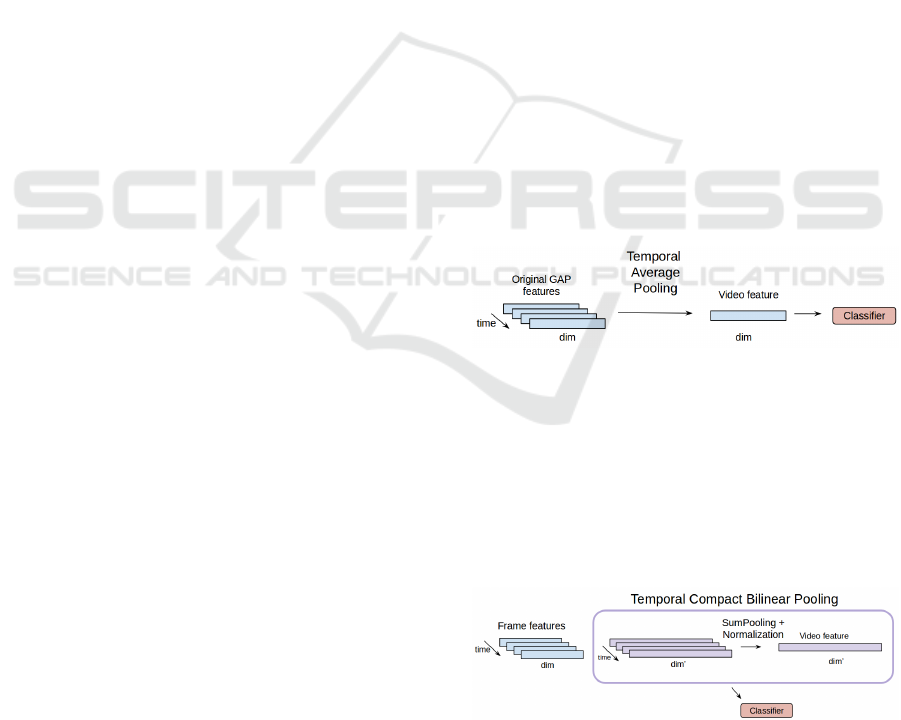
pled frames in a video. Figure 1 illustrates TAP. We
Figure 1: TAP of video frame representations.
propose to use Compact Bilinear Pooling ( CBP ) to
aggregate over the spatial and/or temporal dimension
in video. Temporal Compact Bilinear Pooling ( TCBP )
aggregates information across time: the frame-level
representations at each time point are projected to a
higher dimensional representation using CBP, then are
sum-pooled over the time to generate a global video
representation (see Figure 2).
Figure 2: TCBP of video frame representations.
When processing video clips with a 2D CNN, each
frame independently ignoring the temporal dimen-
sion to produce a representation
ˆ
X ∈ R
t×h×w×c
from
Temporal Bilinear Encoding Network of Audio-visual Features at Low Sampling Rates
639

last convolutional layer, which is then used as input
to TBEN. To transform this into a compact spatial-
temporal representation, the information of
ˆ
X on spa-
tial ( h and w ) and temporal ( t ) dimensions needs to be
aggregated. There are several approaches that could
be used to achieve this. Spatial CBP (SCBP) has been
shown to be more effective than a fully connected
layer to aggregate features from convolution layers in
fine-grained visual recognition tasks (Lin et al., 2015).
SCBP using the RM approximation can be defined as:
f
s
(
ˆ
X) =
|S|
∑
s∈H×W
f
RM
( ˆx
s
), (3)
where f
s
: R
t×h×w×c
→ R
t×c
. Temporal CBP (TCBP)
is defined similarly:
f
t
(
ˆ
X) =
|S|
∑
s∈T
f
RM
( ˆx
s
), (4)
where f
t
: R
t×h×w×c
→ R
h×w×c
. TCBP and SCBP can
act as two independent modules. For example, we can
use SCBP to pool spatial information and then use
TAP or TCBP to aggregate temporal information. We
can also discard SCBP, by just using Global Average
Pooling of last convolutional layer and then apply TAP
or TCBP. Finally, we can also pool spatial-temporal
information using CBP jointly, which we refer to as
STCBP:
f
st
(
ˆ
X) =
|S|
∑
s∈T ×H×W
f
RM
( ˆx
s
), (5)
where f
st
: R
t×h×w×c
→ R
c
. This can give a differ-
ent representation to applying SCBP and then TCBP
(SCBP-TCBP), which is defined as:
f
t
( f
s
(
ˆ
X)) =
|S|
∑
s∈T
f
RM
|S|
∑
s∈H×W
f
RM
( ˆx
s
)
!
, (6)
where f
s
: R
t×h×w×c
→ R
t×c
and f
t
: R
t×c
→ R
c
. To
make the abbreviation clear, we use the notation f
st
(·)
and f
t
( f
s
(·)) for Equation 5 and 6. We also define
f
t
( f
¯s
(·)) , f
¯
t
( f
s
(·)) and f
¯
st
(·) for SAP-TCBP, SCBP-
TAP, and STAP. In our experiments where spatial and
temporal pooling are applied sequentially, spatial pool-
ing is always applied first.
3.2 Hierarchical Label Loss
We explore the label dependency by combining the
classification of coarse and fine-grained categories,
similarly to how it is used in the YOLO object detector
network (Redmon and Farhadi, 2017). Figure 3 shows
an example of fine-grained classes and their parents.
Figure 3: Example illustrating the coarse and fine level
annotations in the FGA-240 dataset.
Parent classes are displayed on the top row and child
classes on the bottom. The joint parent-child class
distribution is given by:
P(A
p
, A
c
) = P(A
c
|A
p
)P(A
p
), (7)
where A
p
is a random variable representing the label
of parent class, A
c
a random variable representing the
label of the child classes, and P(A
p
, A
c
) is the joint
probability of a video being labeled with a particular
parent and child class. The classifier is easily imple-
mented using a fully connected layer of 325 neurons
(240 child and 85 parents), where a softmax normal-
ization is applied on the parent activations to obtain
P(A
p
) (only one parent class is possible per video) ,
and a softmax normalization is applied on the child ac-
tivations to obtain P(A
c
|A
p
) (only one child is possible
per video). The final probability score is obtained by
multiplying parent and child probabilities as in Eq. (7) .
3.3 Decoupled Modalities
Short-term Motion. Many researchers (Carreira
and Zisserman, 2017; Yue-Hei Ng et al., 2015; Varol
et al., 2018) have reported the importance of motion
features, specifically the usefulness of optical flow. Al-
though TBEN is designed to capture and aggregate
long range temporal information, short term motion is
important for distinguishing between certain activities
(e.g. soccer juggling versus soccer penalties). To cap-
ture the very short-term motion and complement the
long-range temporal information captured by TBEN,
we compute optical flow sparsely. Section 4.2 gives
further details.
Audio. Audio is an important cue in videos, yet few
researchers have used it for video classification. VG-
Gish model (Hershey et al., 2017) is used to extract
128D audio embeddings at every second. It takes 0.38s
to extract one minute of audio. Table 1 shows the
performance of the audio modality when setting the
TCBP output dimensions to 512D and 4096D. The
higher dimensional representations of audio perform
better. Audio alone performs significantly worse than
the visual modality ( 23.49 % vs 44.87 % and 44.33 %
Hit@1; see Table 3). Some of the audio is unrelated
to the semantic video content (e.g. musical scores),
which explains the poor performance of audio alone.
VISAPP 2021 - 16th International Conference on Computer Vision Theory and Applications
640

Table 1: Results of TCBP on the audio modality.
Dimension Hit@1 Hit@5
512 19.52 43.17
4096 23.49 47.66
4 EXPERIMENT RESULTS
All single frame models for FGA240 and UCF101 are
sampled at 1 FPS. All experiments in the this and the
following sections are performed on a single NVIDIA
GeForce GTX TITAN X 12GB GPU.
4.1 FGA240
FGA240 is much larger than UCF101, and contains
longer videos. To train classification models in a rea-
sonable length of time, we do not fine-tune the CNNs,
but instead use output of last convolutional layers of
ResNet-50 (He et al., 2016) and Inception-v3 (Szegedy
et al., 2016) as features.
Single Frame Model. We first conduct experiments
on a single frame model. Here, all sampled video
frames are used for training a image classifier. Dur-
ing inference, the average predictions of all frames is
used as the final prediction. The current state-of-the-
art (Sun et al., 2015) on FGA240 uses Alexnet, which
is slightly dated. Our single frame model uses ResNet-
50 and Inception-v3 features and a linear layer with
softmax activation to generate the final predictions.
The linear layer is trained using SGD with momentum
0.9 and learning rate 0.01. Results of single frame
model are report in Table 3.
Average and Bilinear Pooling. Table 2 shows the
results of combinations of average and/or bilinear pool-
ing on spatial and temporal dimensions. The table
shows that AP in both the spatial and temporal di-
mension gives the poorest performance. With ResNet-
50 features CBP on the temporal dimension always
improves performance over AP. With Inception-v3
features, however, the results are less conclusive and
suggest applying CBP in either the spatial or temporal
domain, but not both.
With temporal pooling the training set is reduced
from 9 M features to approx 40 K features. The aggre-
gation also makes inference much faster. The average
length of test videos in FGA240 is ∼ 130 seconds
meaning that during inference, the most computation
time is spent on computing the compact bilinear repre-
sentation, which takes ∼ 2.5 milliseconds per video for
SAP+TCBP; 1 ms/video for SCBP+TAP; 20 ms/video
for STCBP; and 26ms/video for SCBP+TCBP. Once
the representations are computed, the classification for
each video takes under 1 ms.
Table 2: Combination of average pooling and bilinear pool-
ing on the spatial and/or temporal dimension on FGA240
using ResNet-50 and Inception-v3 features.
ResNet-50 Inception-v3
Hit@1 Hit@5 Hit@1 Hit@5
f
¯
st
(·) 42.75 75.85 43.24 76.49
f
t
( f
¯s
(·)) 43.40 76.37 44.33 76.30
f
¯
t
( f
s
(·)) 44.41 77.10 44.08 76.76
f
t
( f
s
(·)) 44.73 77.41 44.00 75.54
Comparison with the State-of-the-Art. Table 3
shows the best results using TBEN using ResNet-50
features and Inception-V3. For ResNet-50 features
the best configuration is to pool both spatial and tem-
poral information with CBP, giving 44.87 % Hit@1
and taking just 22 s/epoch to train. As for Inception-
v3 features, the best performance (Hit@1 44.33% )
using visual features is achieved using SAP and fol-
lowed by TCBP. We use concatenation to combine
audio and visual features and it provides the best re-
sults (Hit@1= 46.6 % and 47.4 %) and greatly boosts
the performance over the individual modalities (Ta-
ble 3, + Audio). For both Hit@1 and Hit@5, the
model with the label hierarchy outperforms the one
without (Table 3, + Hierarchy). If we include TBEN,
audio, and the label hierarchy, we achieve Hit@1 of
47.95 using ResNet-50 and 47.20 using Inception-v3
features, compared with a previous state-of-the-art of
43.40 , while being substantially more computational
efficient.
Comparison with BOVW Encoding. We also com-
pare the performance of TBEN with using other so-
phisticated bag-of-visual-words methods for pooling,
such as VLAD and Fisher Vectors, which are used to
aggregate temporal information using average pooled
spatial features. We randomly sample 30K videos and
for each video sample 100 frames to run k -means or
fit Gaussian mixture models. Table 4 shows the re-
sults of using number of cluster k = 64 and 128 for
VLAD and Fisher vector. We notice that 64 clusters
performs better than 128 for Fisher vectors. This may
be due to the poor convergence of the GMM when
when using 128 components. NetVLAD uses 64 clus-
ters and an output dimension of 4096 . For each video,
300 frames of spatially average pooled ResNet-50 fea-
tures are extracted as input for NetVLAD. The batch
Temporal Bilinear Encoding Network of Audio-visual Features at Low Sampling Rates
641

Table 3: Test performance using ResNet-50 and Inception-V3 features in FGA240. TBEN
∗
uses f
st
(·) and f
t
( f
¯s
(·)) for
ResNet-50 and Inception-V3 representations respectively. R
+
and I
+
represent ResNet-50 and Inception-V3 features.
Dim Hit@1 Hit@5
Time/ Epoch
R
+
I
+
R
+
I
+
Single Frame (SAP) 2048 40.27 42.21 72.26 73.63 c. 0.95h
TBEN
∗
4096 44.87 44.33 77.41 76.30 c. 20s
TBEN + Audio 4608 47.42 46.67 79.59 79.14 c. 20s
TBEN + Hierarchy 4096 45.77 44.50 78.79 78.01 c. 20s
TBEN + Audio + Hierarchy 4608 47.95 47.20 80.73 80.29 c. 50s
LSTM with LAF (Sun et al., 2015) 2048 43.40 74.90 c. 3h
size is set to 20 during training. The remaining train-
ing parameters are set to be the same as Section 4.1.
Table 4 shows that neural network based BOVW meth-
ods such as NetVLAD outperform traditional methods.
When comparing NetVLAD and TBEN, we achieve
inferior Hit@1 and superior Hit@5 by using spatial
AP and then temporal CBP, but TBEN is substantially
faster and this is achieved without trainable encod-
ing parameters. It is possible, however, to achieve
similar Hit@1 performance and superior Hit@5 per-
formance to NetVLAD by using joint spatial-temporal
CBP, but in this case the CBP module has to process
more features: f
st
(·) processes 7 × 7 more features
in the CBP module than f
t
( f
¯s
(·)) resulting in longer
encoding times.
Table 4: Results of VLAD, Fisher Vectors, and NetVLAD en-
coding schemes. Time shown is the average time in seconds
to encode the features for a single video.
k Hit@1 Hit@5 Time (s)
VLAD 64 35.24 68.67 0.059
VLAD 128 35.27 67.57 0.108
FV 64 39.24 73.21 0.023
FV 128 31.51 64.45 0.039
NetVLAD 64 44.61 74.82 0.007
f
t
( f
¯s
(·)) N/A 43.40 76.37 0.002
f
st
(·) N/A 44.87 77.36 0.022
4.2 UCF101
In the training process, we fine-tune the ResNet-50
in an end-to-end manner with TBEN embedded after
feature extraction.
Sampling Rate. We propose a new mid-frame sam-
pling strategy, which only takes the middle frame for
each 1 FPS sampled video during training. During
testing, all frames sampled at 1 FPS are processed,
computing the average of the individual predictions.
Inception V3 is used to train the single frame model
using SGD with a momentum of 0.9 and base layers
of 0.01 on the last linear and auxiliary linear layer and
0.001 elsewhere. The results indicate that, even with
the significant data reduction, we still achieve quite
reasonable accuracy (84.19% in Table 6). To experi-
Table 5: Accuracy of SCBP + TCBP using different sampling
rates on UCF101.
FPS 0.5 1 2 4
SCBP + TCBP 85.75 86.41 84.85 74.02
ment different frame sampling rate, we use 7s sliding
window with stride of 2s in training and 4s in testing.
Table 5 shows the results of using TBEN to aggre-
gate temporal features using different sampling rates.
We see that TBEN does not improve with increased
sampling rates. In fact increasing the sampling rate
to 4 FPS results in a performance decrease of about
10% comparing with 2 FPS. This suggests that TBEN
is good at capturing long range information, but that
small variations between nearby frames might cause
problems.
Comparison with the State-of-the-Art. Following
other state-of-the-art, for motion feature we use optical
flow to encode short-term motion with Farneback’s
dense optical flow (Farneb
¨
ack, 2003) in OpenCV
over 5 consecutive frames using 1FPS sampling rate.
Weights of the backbone network are initialized as
in (Wang et al., 2016). This modality alone achieves
67.19% accuracy. A pretrained VGGish network is
used to extract 128D audio features that are the same
length as the video with 1 descriptor per second. TCBP
is used to aggregate all temporal audio features to
a 1024D representation, achieving 24.09% accuracy.
Each modality: RGB, TSCBP, motion, and audio are
trained independently on one GPU. The final predic-
tions are fused by combining the activations of the
last linear layers. Table 6 lists the boost from each
VISAPP 2021 - 16th International Conference on Computer Vision Theory and Applications
642

modality when we add them in sequential order: RGB,
motion, and audio. Static visual features from the fixed
mid-frame model give approximately a 1% boost on
top of RGB. Adding optical flow gives another 2.67%
boost, which is the largest among the added modali-
ties. Audio features are fast to compute and give an
almost 2% boost. Table 7 lists the state-of-the-art ap-
Table 6: Accuracy on UCF101 using different modalities and
accuracy gains by adding modalities in late fusion. TBEN*
using STCBP with image size 224 × 224.
Split 1 Split 2 Split 3 Mean
TBEN* 85.25 85.22 86.74 85.74
RGB 83.35 84.09 85.12 84.19
OF 66.40 66.60 68.56 67.19
Audio 24.13 24.58 23.57 24.09
All 91.44 90.63 91.02 91.03
+RGB +1.06 +1.23 +0.76 +1.02
+OF +3.25 +2.46 +2.30 +2.67
+Audio +1.88 +1.72 +2.22 +1.94
Table 7: Comparison with the state-of-the-art on UCF101.
∗
are results from split1.
∗∗
uses an image input size of
256 × 256 . ActionVLAD uses a 1 FPS sampling rate and
7-second window. The other settings of ActionVLAD is the
same as the NetVLAD settings used in Section 4.1.
without
Motion
with
Motion
LSTM (Varol et al., 2018) 82.4 92.7
I3D (Carreira and Zisserman, 2017) 84.5
∗
93.4
∗
TSN (Wang et al., 2016) 87.3
∗
94.2
TLE (Diba et al., 2017) 86.9
∗
95.6
CoViAR (Wu et al., 2018) 89.7 94.9
RF (Piergiovanni and Ryoo, 2019) 85.5 94.5
ActionVLAD
∗∗
81.81
∗
87.10
∗
Ours
∗∗
89.7
∗
92.2
∗
Ours 88.9 91.0
proaches on UCF101 dataset. Without motion features
our approach outperforms two stream, I3D, LSTM,
TSN, and TLE. Including motion features, the pro-
posed approach is around 4% less accurate than the
best approach. This shows the importance of using
good motion features; we used fewer frames and faster
dense optical flow, which might be less accurate. We
also emphasize the importance of using audio features
like VGGish, since they are low-dimensional and fast
to extract. We also trained ActionVLAD, which uses
NetVLAD to encode spatial-temporal information, at
a 1 FPS sampling rate, and found that TBEN outper-
formed ActionVLAD under this limited computational
budget.
5 CONCLUSION
We proposed Temporal Bilinear Encoding Network
(TBEN) for encoding long range spatial-temporal in-
formation. We compose two constraints in the experi-
ments, working at 1 FPS and using a single GPU. We
embedded the label hierarchy in the TBEN and con-
ducted experiments on FGA240. We improved upon
the state-of-the-art by applying TBEN on extracted
deep visual features and deep audio features and using
a hierarchical label loss. The result is significantly
faster than the state-of-the-art at training and inference
time. We also use TBEN on UCF101 to compute an
audio-visual embedding. Unfortunately, as there is
no hierarchy information in this dataset, we could not
use the hierarchical loss. Including (1) the mid-frame
selection strategy, and (2) optical flow, gave close to
state-of-the-art results, with only approx. 3% less ac-
curacy than the far more computationally expensive
models.
ACKNOWLEDGEMENTS
This work has emanated from research conducted
with the financial support of Science Foundation Ire-
land (SFI) under grant number SFI/15/SIRG/3283 and
SFI/12/RC/2289 P2.
REFERENCES
Arandjelovic, R., Gronat, P., Torii, A., Pajdla, T., and Sivic,
J. (2016). NetVLAD: CNN architecture for weakly su-
pervised place recognition. In Proceedings of the IEEE
Conference on Computer Vision and Pattern Recogni-
tion, pages 5297–5307.
Arandjelovic, R. and Zisserman, A. (2013). All about VLAD.
In Proceedings of the IEEE Conference on Computer
Vision and Pattern Recognition, pages 1578–1585.
Bilen, H., Fernando, B., Gavves, E., Vedaldi, A., and Gould,
S. (2016). Dynamic image networks for action recog-
nition. In Proceedings of the IEEE Conference on
Computer Vision and Pattern Recognition, pages 3034–
3042.
Carreira, J. and Zisserman, A. (2017). Quo vadis, action
recognition? A new model and the kinetics dataset.
In IEEE Conference on Computer Vision and Pattern
Recognition, pages 4724–4733. IEEE.
Diba, A., Sharma, V., and Van Gool, L. (2017). Deep tem-
poral linear encoding networks. In Proceedings of
the IEEE Conference on Computer Vision and Pattern
Recognition, volume 1.
Fan, L., Huang, W., Gan, C., Ermon, S., Gong, B., and
Huang, J. (2018). End-to-end learning of motion rep-
resentation for video understanding. In Proceedings of
Temporal Bilinear Encoding Network of Audio-visual Features at Low Sampling Rates
643

the IEEE Conference on Computer Vision and Pattern
Recognition, pages 6016–6025.
Farneb
¨
ack, G. (2003). Two-frame motion estimation based
on polynomial expansion. In Scandinavian conference
on Image analysis, pages 363–370. Springer.
Gao, Y., Beijbom, O., Zhang, N., and Darrell, T. (2016).
Compact bilinear pooling. In Proceedings of the IEEE
Conference on Computer Vision and Pattern Recogni-
tion, pages 317–326.
Girdhar, R. and Ramanan, D. (2017). Attentional pooling for
action recognition. In Advances in Neural Information
Processing Systems, pages 34–45.
Girdhar, R., Ramanan, D., Gupta, A., Sivic, J., and Russell,
B. (2017). Actionvlad: Learning spatio-temporal ag-
gregation for action classification. In Proceedings of
the IEEE Conference on Computer Vision and Pattern
Recognition, pages 971–980.
He, K., Zhang, X., Ren, S., and Sun, J. (2016). Deep resid-
ual learning for image recognition. In Proceedings of
the IEEE Conference on Computer Vision and Pattern
Recognition, pages 770–778.
Hershey, S., Chaudhuri, S., Ellis, D. P., Gemmeke, J. F.,
Jansen, A., Moore, R. C., Plakal, M., Platt, D., Saurous,
R. A., Seybold, B., et al. (2017). CNN architectures for
large-scale audio classification. In Acoustics, Speech
and Signal Processing (ICASSP), 2017 IEEE Interna-
tional Conference on, pages 131–135. IEEE.
Hu, J.-F., Zheng, W.-S., Pan, J., Lai, J., and Zhang, J. (2018).
Deep bilinear learning for RGB-D action recognition.
In Proceedings of the European Conference on Com-
puter Vision (ECCV), pages 335–351.
Kar, P. and Karnick, H. (2012). Random feature maps for dot
product kernels. In Artificial Intelligence and Statistics,
pages 583–591.
Karpathy, A., Toderici, G., Shetty, S., Leung, T., Sukthankar,
R., and Fei-Fei, L. (2014). Large-scale video classifi-
cation with convolutional neural networks. In Proceed-
ings of the IEEE Conference on Computer Vision and
Pattern Recognition, pages 1725–1732.
Lin, T.-Y., RoyChowdhury, A., and Maji, S. (2015). Bilinear
CNN models for fine-grained visual recognition. In
Proceedings of the IEEE International Conference on
Computer Vision, pages 1449–1457.
Liu, J., Yuan, Z., and Wang, C. (2018). Towards good prac-
tices for multi-modal fusion in large-scale video classi-
fication. In Proceedings of the European Conference
on Computer Vision (ECCV), pages 0–0.
Pham, N. and Pagh, R. (2013). Fast and scalable polynomial
kernels via explicit feature maps. In Proceedings of
the 19th ACM SIGKDD International Conference on
Knowledge Discovery and Data Mining, pages 239–
247. ACM.
Piergiovanni, A. and Ryoo, M. S. (2019). Representation
flow for action recognition. In Proceedings of the IEEE
Conference on Computer Vision and Pattern Recogni-
tion, pages 9945–9953.
Redmon, J. and Farhadi, A. (2017). Yolo9000: better, faster,
stronger. arXiv preprint.
S
´
anchez, J., Perronnin, F., Mensink, T., and Verbeek, J.
(2013). Image classification with the fisher vector:
Theory and practice. International journal of computer
vision, 105(3):222–245.
Simonyan, K. and Zisserman, A. (2014). Two-stream convo-
lutional networks for action recognition in videos. In
Advances in Neural Information Processing Systems,
pages 568–576.
Soomro, K., Zamir, A. R., and Shah, M. (2012). UCF101:
A dataset of 101 human actions classes from videos in
the wild. arXiv preprint arXiv:1212.0402.
Sun, C., Shetty, S., Sukthankar, R., and Nevatia, R. (2015).
Temporal localization of fine-grained actions in videos
by domain transfer from web images. In Proceedings of
the 23rd ACM International Conference on Multimedia,
pages 371–380. ACM.
Szegedy, C., Vanhoucke, V., Ioffe, S., Shlens, J., and Wojna,
Z. (2016). Rethinking the inception architecture for
computer vision. In Proceedings of the IEEE Con-
ference on Computer Vision and Pattern Recognition,
pages 2818–2826.
Tenenbaum, J. B. and Freeman, W. T. (2000). Separating
style and content with bilinear models. Neural compu-
tation, 12(6):1247–1283.
Tran, D., Bourdev, L., Fergus, R., Torresani, L., and Paluri,
M. (2015). Learning spatiotemporal features with 3d
convolutional networks. In Proceedings of the IEEE
International Conference on Computer Vision, pages
4489–4497.
Tran, D., Ray, J., Shou, Z., Chang, S.-F., and Paluri, M.
(2017). Convnet architecture search for spatiotemporal
feature learning. arXiv preprint arXiv:1708.05038.
Varol, G., Laptev, I., and Schmid, C. (2018). Long-term
temporal convolutions for action recognition. IEEE
Transactions on Pattern Analysis and Machine Intelli-
gence, 40(6):1510–1517.
Wang, L., Xiong, Y., Wang, Z., Qiao, Y., Lin, D., Tang, X.,
and Van Gool, L. (2016). Temporal segment networks:
Towards good practices for deep action recognition.
In European Conference on Computer Vision, pages
20–36. Springer.
Wu, C.-Y., Zaheer, M., Hu, H., Manmatha, R., Smola, A. J.,
and Kr
¨
ahenb
¨
uhl, P. (2018). Compressed video action
recognition. In Proceedings of the IEEE Conference
on Computer Vision and Pattern Recognition, pages
6026–6035.
Yu, C., Zhao, X., Zheng, Q., Zhang, P., and You, X. (2018).
Hierarchical bilinear pooling for fine-grained visual
recognition. In European Conference on Computer
Vision, pages 595–610. Springer.
Yue-Hei Ng, J., Hausknecht, M., Vijayanarasimhan, S.,
Vinyals, O., Monga, R., and Toderici, G. (2015). Be-
yond short snippets: Deep networks for video classi-
fication. In Proceedings of the IEEE Conference on
Computer Vision and Pattern Recognition, pages 4694–
4702.
Zhang, Y., Tang, S., Muandet, K., Jarvers, C., and Neumann,
H. (2019). Local temporal bilinear pooling for fine-
grained action parsing. In The IEEE Conference on
Computer Vision and Pattern Recognition (CVPR).
VISAPP 2021 - 16th International Conference on Computer Vision Theory and Applications
644