
Augmenting Cats and Dogs: Procedural Texturing for Generalized Pet
Tracking
Dominik Borer, Nihat Isik, Jakob Buhmann and Martin Guay
Computer Graphics Laboratory, ETH Z
¨
urich, Switzerland
Keywords:
Mixed and Augmented Reality, Motion Capture.
Abstract:
Cats and dogs being humanity’s favoured domestic pets occupy a large portion of the internet and of our
digital lives. However, augmented reality technology — while becoming pervasive for humans — has so
far mostly left out our beloved pets out of the picture due to limited enabling technology. While there are
well-established learning frameworks for human pose estimation, they mostly rely on large datasets of hand-
labelled images, such as Microsoft’s COCO (Lin et al., 2014) or facebook’s dense pose (G
¨
uler et al., 2018).
Labelling large datasets is time-consuming and expensive, and manually labelling 3D information is difficult
to do consistently. Our solution to these problem is to synthesize highly varied datasets of animals, together
with their corresponding 3D information such as pose. To generalize to various animals and breeds, as well as
to the real-world domain, we leverage domain randomization over traditional dimensions (background, color
variations and image transforms), but as well as with novel procedural appearance variations in breed, age and
species. We evaluate the validity of our approach on various benchmarks, and produced several 3D graphical
augmentations of real world cats and dogs using our fully synthetic approach.
1 INTRODUCTION
Augmented reality has the potential to enhance our
visual experience of the world with both useful and
entertaining information. In the case of animals, we
could imagine sharing localized information about
our pets, or create amusing augmentations of our
favored animals performing stunts, agility parkours
and everyday activities such as interrupting a football
game. Moreover, animal characters in movies could
be tracked and augmented during previs, or motion
captured for CG re-enactment.
In order to be able to augment animals with 3D
graphical objects from a single RGB camera, we need
to be able to automatically estimate the 3D informa-
tion of the animal in the image. Due to extensive vari-
ability in breed, as well as fur appearance and shape,
animals are notoriously challenging to track.
While deep learning has allowed un-precedent
performance in monocular pose estimation, it
has been in large part thanks to large datasets
of hand-labelled images of humans, such as
the COCO (Lin et al., 2014) and the MPII
(Andriluka et al., 2014) datasets. The problem
with these methods is that first it requires vast
amounts of hand labelling efforts, and second it
is quite challenging to hand-label 3D information
consistently. In consequence, it cannot be used
for 3D pose prediction.
In this paper we solve these problems by leverag-
ing the computer graphics toolbox and synthesizing a
large dataset of animals, labelled with full 3D skele-
ton and camera information. We then design and train
a custom deep neural network (DNN) to regress from
image to 3D pose. At run-time, we provide our net-
work with a real-world image, and retrieve the 3D in-
formation, which we use to add 3D graphical objects
on animals such as hats, wings and riders.
The biggest technical challenge with leveraging
synthetic data is to bridge the so-called reality gap:
the pixel-level difference between real world im-
ages and their synthetic counter-parts. DNNs tend
to over-fit onto particular features only seen in the
synthetic domain, and thereby struggle to general-
ize to real world data. To address this problem,
we employ the strategy of domain randomization
(Tobin et al., 2017). Thus in the data generation pro-
cess, we strongly vary dimensions like pose, shape,
texture, background, lighting, and camera viewpoint.
Another technical challenge to reach the desired 3D
augmentations lies in predicting 3D joint orientation
and positions that have a good overlay in the aug-
mented image space. While 2D tracking has shown
impressive results so far, the exact pixel positions are
often lost when going to a 3D pose. We address
122
Borer, D., Isik, N., Buhmann, J. and Guay, M.
Augmenting Cats and Dogs: Procedural Texturing for Generalized Pet Tracking.
DOI: 10.5220/0010333701220132
In Proceedings of the 16th International Joint Conference on Computer Vision, Imaging and Computer Graphics Theory and Applications (VISIGRAPP 2021) - Volume 1: GRAPP, pages
122-132
ISBN: 978-989-758-488-6
Copyright
c
2021 by SCITEPRESS – Science and Technology Publications, Lda. All rights reserved
synthetic data generation
two stage neural network training
use case
optimization augmentation
augmented result
pose data3D assetcapture
neural network pose datasetsynthetic data
2D
3D
46
46
128
image features
46
46
46
46
affinity maps
joint maps
3D pose branch
1024
7
M
N
7(N −1)
3D root branch
subspace
2D pose
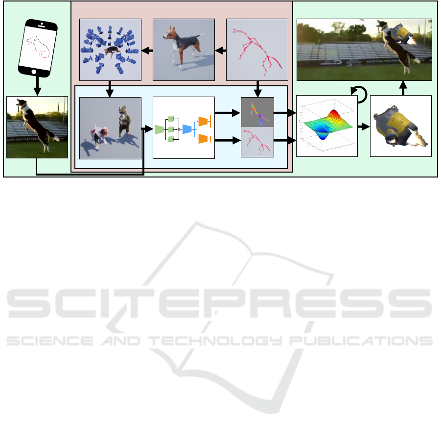
Figure 1: Overview of the proposed approach, which can be divided into 3 basic groups: (red) The data generation process
which allows to create a large dataset of synthetic images with according pose information, 2D and 3D. (blue) The step of
training a neural network to go from synthetic images to the according pose. (green) Using the trained system to predict an
animal’s pose on real world footage, and using those poses to augment the footage with 3D digital assets.
this problem by designing a two step network, pro-
ducing both 2D and 3D information, which can then
be used in an optimization step to create faithful 3D
poses from the camera’s viewpoint. As a result, our
network is able to generalize to real world data and
shows robustness to new environments, shapes, and
appearances. The optimized 3D poses are grounded
in the camera space allowing us to create entertaining
augmentations for cats and dogs in real-world scenar-
ios, as shown in Figure 7.
In Section 4, we discuss the data generation
pipeline, Section 5 addresses the network architec-
ture, and in Section 6 the augmentation of the animals
is explained.
2 RELATED WORK
The vision of digitally augmenting the real
world was first introduced over fifty years ago
(Sutherland, 1968), and has since been revisited
countless times as progress in hardware, computer
vision, and computer graphics continues to be
made — each time unlocking new possibilities for
communication, education and entertainment.
Several augmentation concepts have already
been explored for humans around the body,
face and hair — allowing people to try vir-
tual make-up and glasses (Javornik et al., 2017),
hairs styles (Kemelmacher-Shlizerman, 2016),
and clothing (Rogge et al., 2014, Facecake, 2015,
Yang et al., 2016). To our knowledge, the only pets
augmentation is from SnapChat, which we believe
utilize a combination of 2D feature predictions
together with the phone’s gyroscope to create 3D
augmentation effects, but limited to front-facing dog
faces.
To augment animals with 3D objects, we need
to estimate their 3D pose. Many techniques for
animals build upon methodology developed for hu-
man tracking, more specifically 2D landmark or body
part estimation (Wei et al., 2016, Newell et al., 2016,
Cao et al., 2017, Xiao et al., 2018) from RGB im-
ages. A large dataset of images — typically hand-
labelled with 2D body part locations — is used to
train a multi-stage deep convolutional neural network
(DCNN) to predict the confidence location map of
each joint or landmark; each stage improving the pre-
dictions.
For 3D pose estimation, it is common to train
a separate network to go from 2D-to-3D joint lo-
cations (Chen and Ramanan, 2017, Tom
`
e et al., 2017,
Martinez et al., 2017, Pavllo et al., 2019). We build
upon this work and extend it to our use case of
animal tracking as described in Section 5.2. An-
other line of work extends the convolutional net-
work to predict volumetric 3D joint confidence maps
(Pavlakos et al., 2016, Mehta et al., 2017), and then
optimizes for a kinematic skeleton to match the 3D
predictions (Mehta et al., 2017). However, this ap-
proach lacks limb orientation, and the sparse set of
landmarks can easily loose track of the 3D orienta-
tion of the limbs; which could be attenuated by op-
timizing for a mesh instead of a kinematic skeleton
(Xu et al., 2018).
Seeing the progress in human pose estimation,
biologists have integrated deep learning based ap-
Augmenting Cats and Dogs: Procedural Texturing for Generalized Pet Tracking
123

proaches to track and measure the movements of an-
imals and insects (Kays et al., 2015). Most work in
this area is focused on labelling tools for 2D pre-
dictions (Graving et al., 2019, Pereira et al., 2018).
Some work has focused on modeling the shape of an-
imals (Zuffi et al., 2016) from scans of toy figurines,
optimizing for 3D shapes to match 2D joint esti-
mations (Biggs et al., 2018) and capturing their tex-
ture from video footage (Zuffi et al., 2018). Recent
work combine those approaches in a deep learning
framework to estimate Zebra pose, shape and texture
(Zuffi et al., 2019) or try to leverage the progress in
human pose estimation by transferring it to animals
using domain adaptation (Cao et al., 2019).
To avoid manually labelling images, as
well as to overcome the challenge of labelling
3D information, many works, both for hu-
mans (Chen et al., 2016, Varol et al., 2017,
Xu et al., 2019) and animals (Biggs et al., 2018,
Mu et al., 2019, Zuffi et al., 2019) have explored
generating synthetic datasets.
(Mu et al., 2019) use 3D models to label the im-
ages with 2D landmarks, and devised a learning
scheme to bridge the reality gap. (Chen et al., 2016)
estimate a 3D skeleton from 2D image features, and
they include a domain similarity loss to help steer the
feature extractor extrapolate to real world imagery. To
avoid dealing with the reality gap, (Biggs et al., 2018)
create a dataset of silhouettes and regress from silhou-
ettes to 2D keypoints. This unfortunately only per-
forms as good as the given silhouette estimator.
Another way to address the reality gap is by
so-called domain randomization (Tobin et al., 2017)
— to add noise and variations to the dataset to
avoid over-fitting. Domain randomization has been
shown to achieve state-of-the-art accuracy for car de-
tection (Tremblay et al., 2018, Khirodkar et al., 2018,
Prakash et al., 2019), and has unlocked the possibility
to use in the real world. In this work, we extend this
principle to articulated figures such as animals.
3 OVERVIEW
The core of our approach is a 3D pose predictor from
an RGB image. Our overall approach is summarized
in Figure 1. While deep neural networks provide
state-of-the-art performance for monocular pose es-
timation, several problems must be overcome in order
to be able to track and augment animals.
First, there are no publicly available datasets of
animals labeled with 3D skeletons. To solve the data
problem, we create a highly varied synthetic dataset
of animal images, labeled with 3D information — the
red area in Figure 1. The details of this process are
discussed in Section 4.
Second, directly regressing from the 2D image do-
main to accurate 3D skeletons remains to this day a
challenging task. Two strategies help improve our ac-
curacy (blue area in Figure 1). First to perform as
much processing as possible in the image domain.
Hence we predict 2D joint locations and bone direc-
tions as 2D activation maps (Section 5.1), before re-
gressing to 3D. The second strategy is to avoid unnec-
essary correlations between the 6D rigid (root) pre-
diction and the rest of the body joints, as described in
Section 5.2.
The third problem comes from limited GPU mem-
ory, which does not allow processing large image
frames in real-time. We solve this by estimating a
2D crop when sequentially processing videos. How-
ever, the local crop causes our 3D predictions to be
in many different virtual cameras, as opposed to the
footage-capturing camera. To solve this problem, we
optimize for a 3D skeleton in the footage-capturing
camera space, that seeks to match the 2D predictions,
while remaining as similar as possible to the 3D pre-
dictions, which is detailed in Section 6. Finally at
run-time we attach 3D objects onto the optimized 3D
skeleton, as shown in the green area of Figure 1.
4 DATA GENERATION
Our approach leverages modern computer graphics
to create a realistic dataset of images I labelled with
3D skeleton information X, Q in camera space, with
X representing skeleton coordinates and Q the pose
(represented as quaternions). The main challenge for
creating realistic images of cats and dogs, lies in their
vast variability when it comes to appearance, shape,
pose, lighting conditions, and environment. Thus, for
any learning framework, over-fitting on a specific an-
imal — not to mention on a synthetic one — is a se-
rious challenge. Additionally, due to the approximate
nature of the 3D assets and the rendering algorithms,
the learning framework is challenged by a so-called
domain gap, i.e. the difference between the synthetic
training data to the real world test data.
To address the domain gap and over-fitting prob-
lems, we leverage the principle of domain ran-
domization (Tobin et al., 2017, Tremblay et al., 2018,
Khirodkar et al., 2018). Hence, we programmatically
introduce a large amount of variability in the most sig-
nificant dimensions of the dataset, i.e. texture, shape,
pose, lighting, and context (or scene background).
This domain randomization can be seen as a reg-
ularization or alternatively, as as a vast expansion of
GRAPP 2021 - 16th International Conference on Computer Graphics Theory and Applications
124
scene and camera
poses
blendshapes
materials
appearance3D model
rendered data
image augmentation
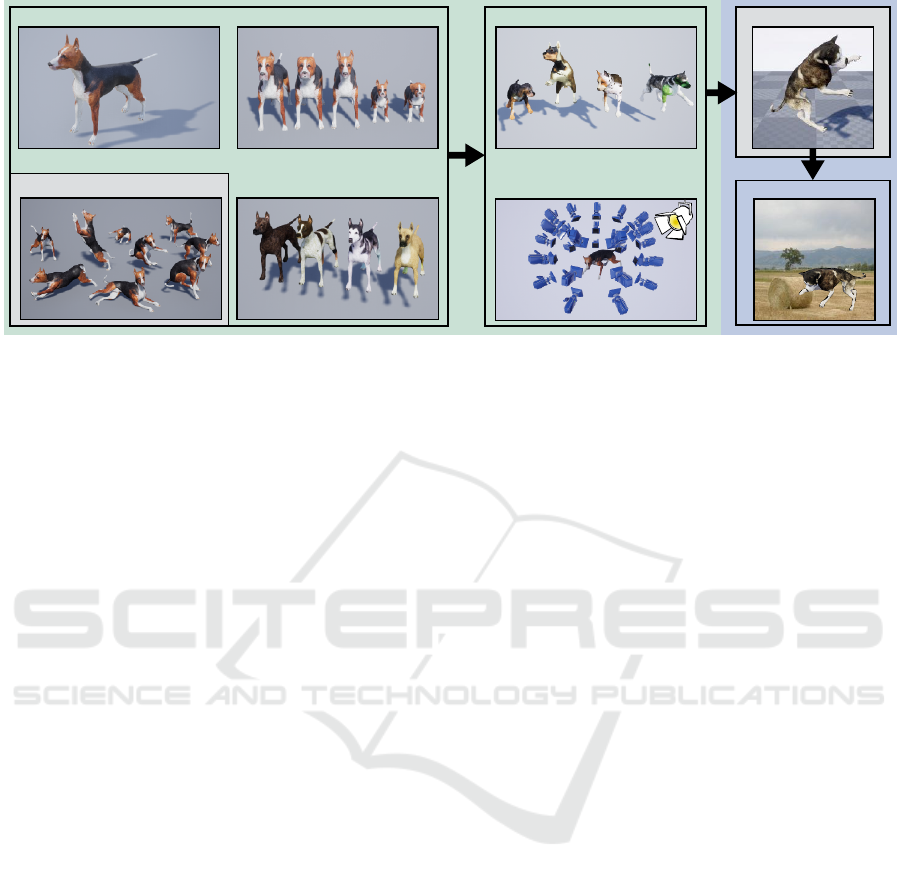
a) asset selection b) randomization c) training data
Figure 2: Overview of the data generation pipeline: The pipeline can be split in a 3D part (green) and a 2D part (blue): a) a 3D
asset (including mesh, blendshapes, poses, materials), and b) a randomization process where those components are sampled
to create a large variation of appearances. Additionally, the scene and camera settings are sampled, leading to the rendered
images that are stored together with the pose data (grey). c) During training, standard image augmentations are applied in
image space.
the training data distribution that reduces the distance
to the real world distribution. Randomizing shape,
pose, appearance and lighting requires 3D informa-
tion and is therefore applied during the animal ren-
dering procedure (Section 4.1). Besides this 3D ran-
domization we apply standard 2D image augmenta-
tion techniques such as color space transforms and 2D
geometric transforms during training directly in im-
age space (Section 4.2). Without the 2D/3D random-
ization the model would overfit to the few synthetic
animals and not generalize to images of real animals.
The overall data generation process is summarized in
Figure 2.
4.1 3D Randomization
We utilize a 3D game engine for fast rendering and
fast iterations over our datasets. For this purpose,
we parameterize the shape and pose of animals with
parameters β and Q respectively for shape and pose.
Such a parameterization is compatible with real-time
game engine rigs, which typically offer only blend
shapes and linear blend skinning (LBS) as shape pa-
rameterizations.
4.1.1 Shape Parameterization
Our approach starts with a 3D mesh of an animal in
a rest pose V
0
, whose shape variations ∆V
j
( j differ-
ent entire meshes) have been hand-crafted for differ-
ent breeds, age, muscle, fat, bone, etc. We purchased
these models on the DAZ platform (DAZ, 2019).
Unlike a small local shape variation such as a
muscle bulge, our shape variations for breed and age
affect the entire proportions of the mesh, including
its underlying skeleton. Hence to remain compatible
with LBS, we parameterize the skeleton coordinates
X w.r.t. surrounding mesh vertices, which are being
deformed by blend shape parameters β
j
as follows:
V = V
0
+
∑
j
β
j
∆V
j
. For each joint i we choose to lin-
early map the L closest vertices V
i
to the joint position
x
i
. Hence, we take those mesh vertices in the rest pose
V
i
0
with the corresponding joint position x
i
0
and solve
a linear least squares problem: kA
i
V
i
0
+ b
i
− x
i
0
k w.r.t.
A
i
and b
i
. Given a deformed mesh V , the joint posi-
tions can then be determined as: x
i
= A
i
V
i
+ b
i
, using
the precomputed A
i
and b
i
.
Following our principles of domain randomiza-
tion, we sample shape parameters β in a broad range,
which not only cover the original artist-intended
species, but also various blends between them.
4.1.2 Pose Sampling
In order to robustly track animals in their everyday
life, the training data needs to reflect the poses ani-
mals tend to perform. Since motion capturing animals
is cumbersome, expensive and often times danger-
ous, we pursue a strategy to leveraging only a sparse
set of poses, such as a hand-crafted dataset of about
200 distinct poses; purchased on the DAZ platform
(DAZ, 2019).
To sample pose variations, we model a pose dis-
tribution using principal component analysis (PCA).
The resulting pose vector is then sampled as Q = P ·t
Augmenting Cats and Dogs: Procedural Texturing for Generalized Pet Tracking
125
where P reflects the first K dimensions of the PCA de-
composition and t is sampled from a K dimensional
multivariate Gaussian.
4.1.3 Appearance Sampling
Naively applying random textures to the appearance
of animals will cause the network to disregard impor-
tant visual cues that appear in texture and help predict
the pose, such as the line between the face color and
the fur. Hence one can obtain much better results by
creating new textures from existing ones — assuming
multiple textures in correspondence — by blending
between the textures in a seamingly natural way, e.g.
part Dalmation and part German Shepherd.
Since uniformly interpolating between two tex-
tures leads to washed out colors of both textures, we
model texture blending via local patches. We syn-
thesize a 2D blend map R
2
→ R
1
using a percep-
tually natural noise distribution such as Perlin noise
(Perlin, 2002). This blending approximates spatially
smooth patchwork of species variations in our appear-
ance textures, cf. Figure 2b).
Although our textures do not always exist in the
real world, we found that this kind of randomiza-
tion helps generalizing to new animal appearances not
present in the training dataset. Note that we add varia-
tions in color space to the rendered images during the
training, as detailed later in Section 4.2.
4.1.4 Viewpoint Sampling and Rendering
Lastly, the camera and scene elements such as lights
and occluders are sampled.
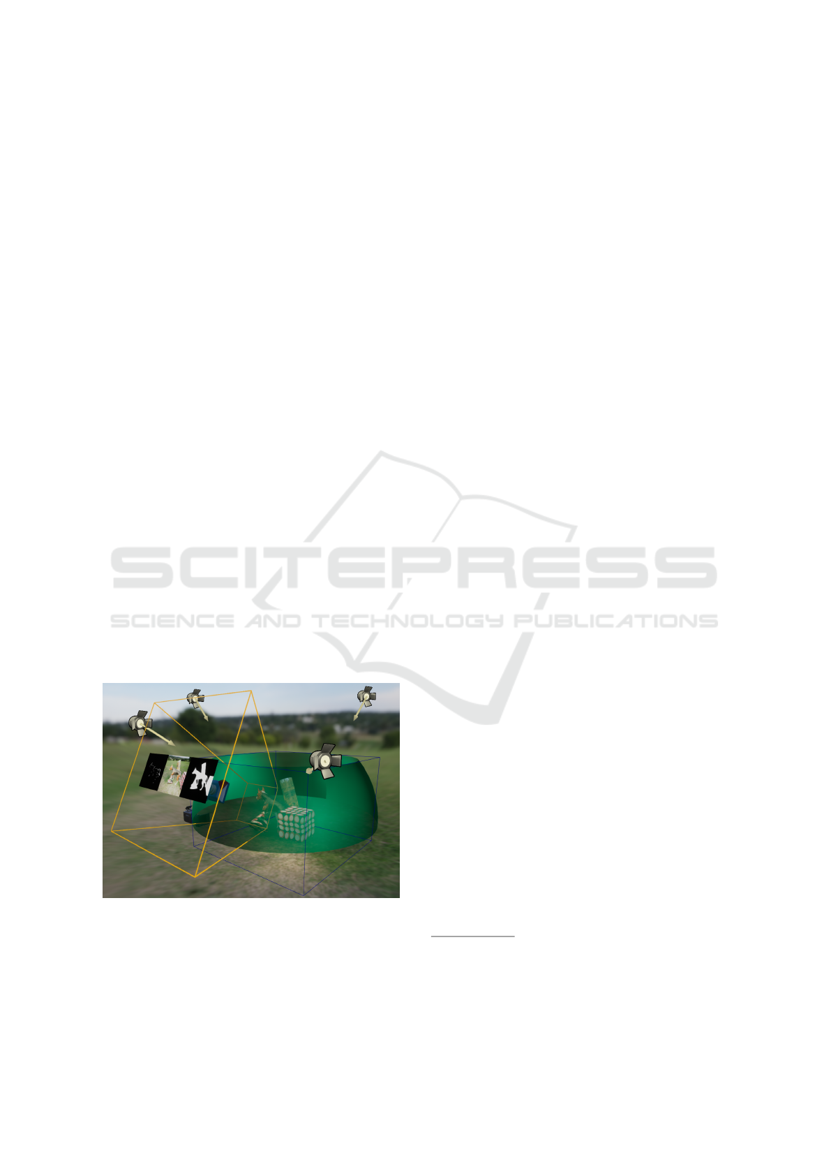
Figure 3: Overview of the render setup: The camera is sam-
pled on the green surface, and then varied within the yellow
volume, random meshes are spawned as occluders within
the blue capture volume and different light sources are ran-
domized.
Camera. The camera location is sampled on a
sphere around the animal with a fixed radius and con-
straints on azimuth and elevation, illustrated with a
green shape in Figure 3. This position then defines
the camera orientation, which is aligned with the root
of the 3D skeleton. Additionally, a positional offset is
sampled in a predefined volume around the camera
location, aligned with the camera orientation, (yel-
low volume in Figure 3) to get the final camera po-
sition. Lastly, the camera orientation is varied in a
small range to get more out-of-center views.
Lighting. We vary light sources, by sampling col-
ors, intensity, as well as light type between point-
and spotlight. Additionally, multiple skylights are
blended to achieve a more natural illumination.
Occluders. To be robust to missing body parts, we
add occluders defined as random meshes floating in
the scene. Their position in the capture space, as well
as their orientation, scale, color, and texture is sam-
pled from a predefined range.
4.1.5 Labels
Finally, the image features (RGB-image and mask)
are rendered at the desired resolution and saved to
disk. The pose parameters Q and the skeleton posi-
tions X are mapped into a space relative to the camera.
These composed values are then saved together with
the camera coordinates, the projection parameters, as
well as the 2D coordinates of the skeleton joints.
4.2 2D Randomization
To avoid over-fitting on a specific background, we
randomize the context in which animals may appear.
We sample random backgrounds, composed with the
rendered animal using its 2D mask. The backgrounds
are images of natural environments, as well as urban
and office settings.
Once overlayed onto a background, the image is
further randomized with color space transformations,
to account for different brightness, hue, saturation,
blur, pixel noise, as well as with geometric transfor-
mations such as translation, rotation, scaling and mir-
roring. Note that we transform the labels according
to the geometric transform to maintain the correspon-
dence.
1
1
Note that the set of geometric transforms changes de-
pending on which part of the system is trained (2D vs. 3D),
because not all 2D transforms in the image plane can be
faithfully mapped to a corresponding transform on the 3D
labels.
GRAPP 2021 - 16th International Conference on Computer Graphics Theory and Applications
126
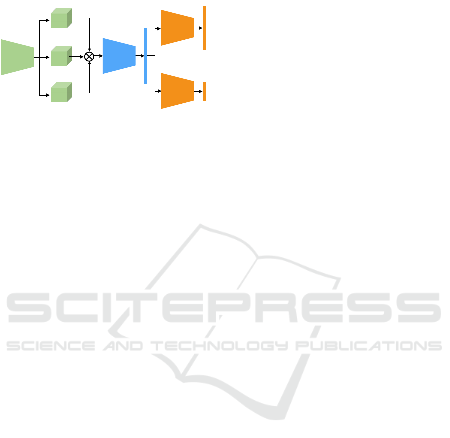
46
46
128
image features
46
46
46
46
affinity maps
joint maps
3D pose branch
1024
7
M
N
7(N −1)
3D root branch
subspace
2D pose
Figure 4: Neural network architecture overview, which con-
sists of three building blocks. First a 2D system (green)
that takes images as input and predicts 2D feature maps.
Those features are concatenated and with multiple convo-
lutional layers reduced to a lower dimensional subspace
(blue). Lastly, two branches (orange) map the subspace to
the 3D pose information, with one branch for the root and
another for all other joints in a body-centric fashion. Train-
ing is done in a two-stage manner: first the 2D part is trained
until convergence, before the full system is trained.
5 NETWORK ARCHITECTURE
The result of the data generation process is a dataset
of RGB images I of animals at resolution 368 × 368,
together with their corresponding 2D pixel coordi-
nates P
X
= {p
1
, ..., p
N
}, and 3D labels {X, Q} =
{x
1
, q
1
, ..., x
N
, q
N
}, with N being the number of joints.
This data allows us to design a deep neural network
and train it to predict 3D skeleton poses from an input
image.
While DNNs have progressed rapidly in recent
years, it remains a challenge to regress directly from
the image domain to 3D skeletons. Hence we break
the problem down into 2D pose feature predictions of
2D joint confidences I
C
and 2D joint affinities I
A
at
resolutions 46 × 46, followed by a module that con-
catenates the 2D features and predicts a 3D skeleton
pose X , Q. An overview of this architecture is shown
in Figure 4. Examples of joint confidence and affinity
maps can be seen in Figure 5 and Figure 6.
5.1 2D Pose Estimation
The 2D part of our network follows the architecture
of (Cao et al., 2018), which consists first of a pre-
trained feature extractor backbone (in our case VGG
(Simonyan and Zisserman, 2015) pre-trained on Im-
ageNet (Deng et al., 2009)), followed by a multi
stage convolutional neural network, that refines the
predictions over successive stages, with interme-
diate supervision at each stage (Wei et al., 2016,
Cao et al., 2017, Cao et al., 2018). Each stage out-
puts joint confidence and affinity maps I
C
pred
, I
A
pred
and
using the ground truth maps I
C
gt
, I
A
gt
we minimize for
training the L2 loss:
L (I
C
, I
A
) =
I
C
pred
− I
C
gt
2
2
+
I
A
pred
− I
A
gt
2
2
. (1)
5.2 3D Pose Estimation
After the 2D stage, we concatenate the predicted
joint confidence maps I
C
46×46×N
with the affinity maps
I
A
46×46×M
, where M is the number of predicted bones,
and the image features I
F
46×46×128
extracted with the
pre-trained feature extractor, and feed them to our
3D-predicting module, which outputs a fixed size 3D
skeleton pose vector X, Q.
To avoid learning unnecessary correlations be-
tween root and the rest of the pose, we separate the
network into two dedicated branches: one for the root,
and one for the joints.
In a first step, the concatenated image features and
the predicted 2D feature maps are mapped to a lower
dimensional latent space (1 × 1 × 1024) using convo-
lutional blocks each reducing the spatial dimensional-
ity of the features (4x4 convolutions, with stride 2 and
padding 2, followed by batch norm and leaky ReLu
with slope 0.2). We then feed the fixed size latent vec-
tor to the two separate branches (for root and pose),
which each have the same fully connected (FC) archi-
tecture.
The FC branches follow a resnet type of archi-
tecture similar to (Martinez et al., 2017), where lin-
ear layers followed by ReLu activation functions are
combined with their residual from the previous layer
to map to the dimensionality of the pose vector, as
shown in Figure 4.
To train the 3D module, we minimize two losses:
one for 3D positions X, and one for the orientations
Q. Since the orientations are represented as quater-
nions, we choose an angular distance d
Q
pred
, Q
gt
=
arccos
Q
pred
, Q
gt
, as it is differentiable.
L (X, Q) =
X
pred
− X
gt
2
2
+ λ · d
Q
pred
, Q
gt
, (2)
where the weighting λ makes sure that both terms are
equally weighted.
5.3 Training Details
Data Details. In order to reduce redundancies of
pose and viewpoints, the pose data is not represented
in global world coordinates, but transformed into
camera coordinates. Additionally, the pose is rep-
resented in a body frame representation, which fac-
tors out the root position and orientation for all other
joints. Hence, the same pose in different positions and
Augmenting Cats and Dogs: Procedural Texturing for Generalized Pet Tracking
127
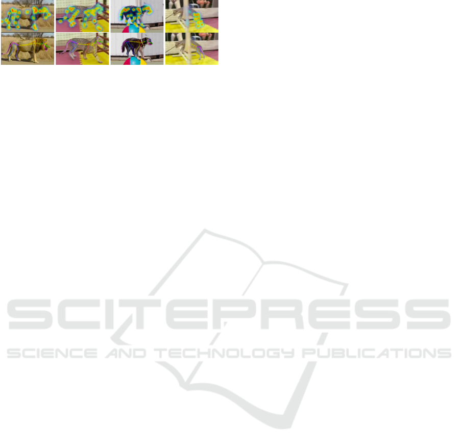
Figure 5: Example outputs of the 2D network (joint maps
on top) and the inferred 2D skeleton (bottom). The most
right example shows a common problem with occlusions
which can easily occurs for animals the size of a cat.
root orientations does not vary. Note, the body frame
representation also leads to a decoupling of the cost
and thereby the gradients in the two branches. To get
back to the camera space, the predicted joint positions
and orientations are combined with the predicted root
pose, as follows:
b
X
i
= X
root
pred
+ X
i
pred
and
b
Q
i
= Q
root
pred
· Q
i
pred
. (3)
Hardware and Learning Settings. We generate
a dataset of 100k samples, covering a wide range
of randomizations. The 3D positions and orienta-
tions are normalized to zero mean and unit stan-
dard deviation, the input images are normalized
using the pre-computed statistics from ImageNet
(Deng et al., 2009) and the joint- and affinity-maps
are not normalized. Each model, 2D and 3D, is then
trained on the entire dataset for 100 epochs, using the
Adam optimizer (Kingma and Ba, 2015) with an ini-
tial learning rate of 1e-4, and a decay factor of 0.5
every 20 epochs, with a mini-batch of size 16. The
training of each module takes about three days on an
NVIDIA Titan Xp (12GB).
6 TRACKING AND
AUGMENTATION
Taking an image as input, our network outputs 2D fea-
ture maps (joint confidence maps I
C
and affinity maps
I
A
), together with a 3D skeleton of the pose X, Q.
There are two challenges that prevent us from directly
using the 3D pose for augmenting graphical elements.
The first is that our model was trained specifically for
images of size 368 × 368 (capped by current GPUs
memory size) and we cannot track an animal in a full
larger frame. The second aspect is how deep neural
networks map the 3D space. It behaves in a near-
est neighbor fashion leading to 3D predictions which
seem natural, but are not “spot on” with regard to the
joints in image space.
To solve these challenges, we first utilize a crop to
track in a full image space, and then perform an op-
timization in 3D for a pose that matches best the 2D
features, while remaining close to the 3D pose in our
crop. Note that optimizing directly for 2D predictions
would cause spurious poses due to a lack of 3D con-
straints, and would be challenged by global detection
(prediction of the overall orientation of the body and
limbs).
Assuming a run-time frame is of size
ˆ
I
1920×1080
.
At the first frame, we utilize the fully convolutional
part of our network which predicts the 2D maps, and
estimate a crop position and size. The subsequent
frames
ˆ
I(t) will use the previous frame’s
ˆ
I(t − 1) pre-
dictions to predict the next crop.
Using the crop, we feed the cropped image
to our network and retrieve the 3D pose X, Q,
as well as the 2D feature maps I
C
, I
A
. Using
the feature maps and the graph-based inference of
(Cao et al., 2017), we compute 2D skeleton joint po-
sitions
b
P
X
= {p
1
, ..., p
N
} in the full image space. Now
we solve for a new pose Q
0
and root position X
0
root
as to be similar to the 3D predictions, while con-
forming to the 2D predictions as much as possible
w.r.t. the projected 3D joint locations in image space
Pro j (Φ(Q
0
, X
0
root
):
argmin
Q
0
,X
0
root
Pro j
Φ(Q
0
, X
0
root
)
−
b
P
X
+ λ
Q
· d
Q, Q
0
,
(4)
where Φ(Q) computes the positions P
X
through for-
ward kinematics (bone lengths are determined from
the predicted positions X).
6.1 Graphics Augmentation
With the 3D skeleton, we can attach rigid objects to
joints and transform them using the joint position and
orientation.
We scale the object based on the average depth of
the skeleton, and length of the body defined as the
pelvis joint to the neck joint.
Rigid objects in their identity transform may not
be aligned with the body’s features. For example, a
hat needs to be aligned with the head and oriented as
to be sitting on the head. We utilize a template model
that we dress with all types of augmentations: a hat,
a rider, etc. We pose the object into a transform
b
T (0),
and then compute the transform between the template
rig transform and the object’s transform, resulting in
T
−1
(0)
b
T (0).
At runtime, we have a predicted joint transform
T (t) and the objects position and orientation is thus:
b
T (t) = T (t)T
−1
(0)
b
T (0).
GRAPP 2021 - 16th International Conference on Computer Graphics Theory and Applications
128
joint maps affinity maps inferred 2D skeleton predicted 3D skeleton tracked 3D skeleton augmented image
Figure 6: Overview of the different intermediate results along the system.
7 RESULTS AND DISCUSSION
7.1 Data
Using our data generation pipeline, we were able to
generate seemingly realistic images of animals cover-
ing a wide and diverse range of variations, as shown
in Figure 2 and accompanying video. Our new and
diverse dataset allowed us to successfully train a neu-
ral network that is capable of generalizing to real —
never seen before — images of animals. One of the
keys to our success is the flexibility and speed of
our approach, which allowed us to iterate quickly our
data. We experimented with both a dog dataset com-
prised of German shepherd, wolf, bull terrier, etc., and
a dataset of felines comprised of lion, tiger, cheetah,
etc. We trained models on each individual dataset, as
well as on mix of both (dog and cat). While the mod-
els from the individual datasets perform well for the
respective species, the mixed dataset outperformed
both, which further strengthens the principle of do-
main randomization.
7.2 Network
The 2D pose estimation part of our network (green
part in Figure 4) is capable of predicting qualitatively
accurately various dog breeds and feline species, both
seen and unseen in our training data. As can be seen
in the first three columns of Figure 5 and in Figure 6,
the 2D predictions of the joint confidence and affinity
maps, as well as the resulting inferred 2D skeleton,
have an accurate overlap with the body parts in the
image. But large occlusions can still be problematic
as can be seen in the last column in Figure 5.
The 3D pose estimation part (blue and orange part
in Figure 4) is still challenging, especially when the
pose space is hard to model. Due to the lack of large
amounts of pose data (for example mocap), we syn-
thetically increased the pose space by vastly sampling
a PCA space, created from our 200 pose samples.
Hence, while the predicted 3D poses still lack in per-
fect overlap with the images, they clearly reflect the
overall action of the animal, as we can seen in the 3D
plot of Figure 6.
Finally, it is worth mentioning that splitting up the
training into two parts: first the 2D part of the net-
work, followed by the 3D part, was crucial. Training
the entire model end-to-end did not converge to the
same level of accuracy.
7.3 Augmentations
One of the main benefits of our network and dataset is
that we can predict not only 3D positions, but also 3D
orientations of the body parts. Hence we can create
graphical augmentations with objects that both move
and rotate along the animal, which was never seen be-
fore — as shown in our accompanying video and Fig-
ure 7.
For example, we thought that if a cat running on
a football field was entertaining enough to make the
news, it would be even funnier once augmented with
a football helmet on its head and a jet-pack on its
spine. We can see on social media people posting vast
amounts of videos with their dog performing stunts or
agility parkour. For example, someone might throw
an object and have their dog catch it in mid-air. We
augmented such stunts with a jet pack, worn on the
back, and with animated angel wings, making it seem
like the dog could fly.
To demonstrate the possibility of exhibiting sec-
ondary dynamics onto another object, we added a
cowboy rider onto a white cat as to look like he is
performing rodeo. The rider is modelled as an artic-
ulated character with elastic dynamics on the joints
with decreasing stiffness as we get further away from
the hip joints. As the cat spine moves and rotates, the
rider follows in a delayed fashion.
7.4 Evaluation
The lack of large public animal datasets limit the op-
tions for quantitative evaluation and comparison to re-
lated work. The two animal datasets we are aware
of (Biggs et al., 2018, Cao et al., 2019), are both rel-
atively small and only provide 2D annotations. Our
Augmenting Cats and Dogs: Procedural Texturing for Generalized Pet Tracking
129
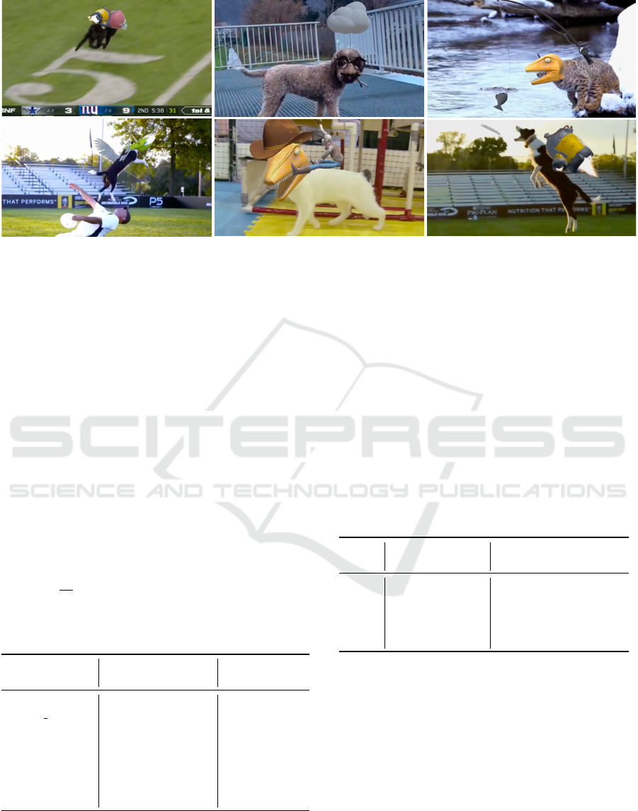
Figure 7: Augmentation results on a variety of dogs and cats performing everyday activities including stunts with their beloved
owners.
skeleton has more joints and hence we can only com-
pare on a subset, which includes 3 joints per leg and
the tail and the facial keypoints, ignoring head, neck,
spine, shoulders and hips. The small discrepancies in
the exact positioning of joints cause additional evalu-
ation errors. Despite having trained only on dogs and
felines, for completeness we evaluate on all provided
animal categories.
The first dataset (Biggs et al., 2018) consists of
short video sequences of various animals annotated
with keypoints and silhouette. While their approach
requires a silhouette extractor, our model predicts
from the raw image. As can be seen in Table 1, for the
dog sequences we outperform their raw confidence
map result and achieve similar accuracy as their op-
timized result.
Table 1: Comparison to (Biggs et al., 2018) using the Per-
centage of Correkt Keypoints (PCK) metric, with threshold
d = 0.2 ·
p
|S|, where |S| is the area of the silhouette. While
their confidence map result (Raw) is further optimized us-
ing using quadratic programming (QP) or genetic algorithm
(GA), our result comes from the graph based inference.
(Biggs et al., 2018) Ours
Raw QP GA All Visible
dog 66.9 66.6 66.9 70.5 77.5
rs dog 64.2 63.4 81.2 77.0 79.6
bear 83.1 83.7 88.9 79.4 85.9
camel 73.3 74.1 87.1 56.6 39.2
cow 89.2 88.4 94.7 80.8 90.6
horsejump-high 26.5 27.7 24.4 50.6 53.9
horsejump-low 26.9 27.0 31.9 50.0 51.6
impala - - - 86.4 86.4
The second dataset (Cao et al., 2019) is based
on Pascal VOC 2011 (Everingham et al., ), extended
with keypoint annotations for various animal cate-
gories. While their approach requires a large-scale
human pose dataset, a smaller animal pose dataset and
an animal bounding box dataset, our approach only
requires synthetic data, which is much cheaper to cre-
ate than an, albeit small, real animal pose dataset. As
can be seen in Table 2, for the dog dataset we achieve
similar performance.
Table 2: Comparison to (Cao et al., 2019) using the Mean
Average Precision (mAP) metric. While for the dog dataset
we achieve similar performance, it does not generalize as
well to other categories. The cat dataset consits of a lot of
very closeup views and furry cats, which differs from our
synthetic data, and hence explains the low performance. For
other categories the error can be explained due to missing
predictions rather than incorrect predictions.
(Cao et al., 2019)
mAP
@0.5 @0.75 Total
dog 41.0 62.9 37.9 38.9
cat 42.3 31.1 13.1 15.0
sheep 54.7 48.3 32.6 33.0
cow 57.3 36.1 17.2 18.4
horse 53.1 60.2 40.2 38.0
Note that the PCK metric only measures the accu-
racy of the predicted keypoints, while mAP also con-
siders missed predictions, which explains the differ-
ence between the two datasets.
Due to the lack of 3D annotations, we evaluate our
model on unseen synthetic sequences. As can be seen
in Table 3, for synthetic data the 2D estimator is ex-
tremely accurate, while the 3D estimator still suffers
from significant errors, especially when the animal is
turning away/towards the camera, compared to a sim-
pler side view.
GRAPP 2021 - 16th International Conference on Computer Graphics Theory and Applications
130
Table 3: Evaluation on unseen synthetic sequences. For the
2D evaluation we use the PCKh metric, where the head seg-
ment spans from the back of the head to the tip of the nose,
and to evaluate the 3D performance we report the Mean Per
Joint Position Error (MPJPE).
2D, PCKh
3D, MPJPE
@1.0 @0.5 @0.1
Walking 99.2 98.6 86.4 19.3
Running 99.9 99.5 90.6 19.3
Sprinting 99.5 98.9 87.5 18.1
Turning 99.5 98.1 79.9 47.8
7.5 Discussion
While we were able to automatically augment many
videos of animals, there remains much room for im-
provement. For example, our predictions still suf-
fer from complex occlusions, motion blur, or from
a large discrepancy with the breeds we used in our
datasets. For instance, presenting an extremely furry
dog caused our network to produce spurious predic-
tions.
Predicting 3D poses from 2D image features such
that the predicted 3D joints overlap accurately with
the 2D body in the image, remains a challenge in com-
puter vision. The 3D predictions are often “smoothed
out” and seem to hold a strong bias towards the mean
pose. Most trackers will then correct this with an op-
timizer as a post process — as we did in this work. In
the future, it would be better to have a cross domain
(pixel to pose) capabilities as to facilitate or even re-
move the last refinement step.
We currently estimate 2D joint confidence maps
in a bottom up fashion, but consider only and trained
only for individual 3D poses. Moving forward, it
would be interesting to track and augment multiple
animals in a scene.
Finally, our synthetic data generates not only 3D
poses, but also UV maps, normals, depth, as well as
mesh vertices. In the future we would like to explore
techniques that can leverage this dense information,
as well as texture-related augmented reality.
8 CONCLUSION
By fully pursuing the principles of domain random-
ization, we procedurally synthesized a large dataset
of cats and dogs with many variations in breeds and
species, and were able to demonstrate the possibility
of automatically tracking and augmenting real world
animals, with synthetic data only — no animals were
hurt in the making of this experiment. In the future,
we would like to improve the accuracy of our 3D pre-
dictions and conceive more compact models deploy-
able on mobile devices.
REFERENCES
Andriluka, M., Pishchulin, L., Gehler, P., and Schiele, B.
(2014). 2d human pose estimation: New benchmark
and state of the art analysis. In IEEE Conference on
Computer Vision and Pattern Recognition (CVPR).
Biggs, B., Roddick, T., Fitzgibbon, A., and Cipolla, R.
(2018). Creatures great and SMAL: Recovering the
shape and motion of animals from video. In ACCV.
Cao, J., Tang, H., Fang, H.-S., Shen, X., Lu, C., and Tai, Y.-
W. (2019). Cross-domain adaptation for animal pose
estimation. In The IEEE International Conference on
Computer Vision (ICCV).
Cao, Z., Hidalgo, G., Simon, T., Wei, S., and Sheikh,
Y. (2018). Openpose: Realtime multi-person 2d
pose estimation using part affinity fields. CoRR,
abs/1812.08008.
Cao, Z., Simon, T., Wei, S.-E., and Sheikh, Y. (2017). Real-
time multi-person 2d pose estimation using part affin-
ity fields. In CVPR.
Chen, C.-H. and Ramanan, D. (2017). 3d human pose esti-
mation = 2d pose estimation + matching. 2017 IEEE
Conference on Computer Vision and Pattern Recogni-
tion (CVPR), pages 5759–5767.
Chen, W., Wang, H., Li, Y., Su, H., Tu, C., Lischinski,
D., Cohen-Or, D., and Chen, B. (2016). Synthesizing
training images for boosting human 3d pose estima-
tion. CoRR, abs/1604.02703.
DAZ (2019). Daz big cat 2 and millennium dog.
https://www.daz3d.com/daz-big-cat-2, https://www.
daz3d.com/mighty-king-poses-for-the-daz-lion,
https://www.daz3d.com/millennium-dog-bundle,
https://www.daz3d.com/ultimate-canine-bundle.
Deng, J., Dong, W., Socher, R., Li, L.-J., Li, K., and Fei-
Fei, L. (2009). ImageNet: A Large-Scale Hierarchical
Image Database. In CVPR09.
Everingham, M., Van Gool, L., Williams, C. K. I.,
Winn, J., and Zisserman, A. The PASCAL Vi-
sual Object Classes Challenge 2011 (VOC2011)
Results. http://www.pascal-network.org/challenges/
VOC/voc2011/workshop/index.html.
Facecake (2015). Swivel.
Graving, J. M., Chae, D., Naik, H., Li, L., Koger, B., Costel-
loe, B. R., and Couzin, I. D. (2019). Fast and robust
animal pose estimation. bioRxiv.
G
¨
uler, R. A., Neverova, N., and Kokkinos, I. (2018). Dense-
pose: Dense human pose estimation in the wild. In
Proceedings of the IEEE Conference on Computer Vi-
sion and Pattern Recognition, pages 7297–7306.
Javornik, A., Rogers, Y., Gander, D., and Moutinho, A. M.
(2017). Magicface: Stepping into character through
an augmented reality mirror. In Proceedings of the
2017 CHI Conference on Human Factors in Comput-
ing Systems, CHI ’17, pages 4838–4849.
Augmenting Cats and Dogs: Procedural Texturing for Generalized Pet Tracking
131

Kays, R., Crofoot, M. C., Jetz, W., and Wikelski, M. (2015).
Terrestrial animal tracking as an eye on life and planet.
Science, 348(6240).
Kemelmacher-Shlizerman, I. (2016). Transfiguring por-
traits. ACM Trans. Graph., 35:94:1–94:8.
Khirodkar, R., Yoo, D., and Kitani, K. M. (2018). Do-
main randomization for scene-specific car detection
and pose estimation. CoRR, abs/1811.05939.
Kingma, D. P. and Ba, J. (2015). Adam: A method for
stochastic optimization. In 3rd International Confer-
ence on Learning Representations, ICLR 2015, San
Diego, CA, USA, May 7-9, 2015.
Lin, T.-Y., Maire, M., Belongie, S., Hays, J., Perona, P.,
Ramanan, D., Doll
´
ar, P., and Zitnick, C. L. (2014).
Microsoft coco: Common objects in context. In Euro-
pean conference on computer vision, pages 740–755.
Springer.
Martinez, J., Hossain, R., Romero, J., and Little, J. J.
(2017). A simple yet effective baseline for 3d human
pose estimation. 2017 IEEE International Conference
on Computer Vision (ICCV), pages 2659–2668.
Mehta, D., Sridhar, S., Sotnychenko, O., Rhodin, H.,
Shafiei, M., Seidel, H.-P., Xu, W., Casas, D., and
Theobalt, C. (2017). Vnect: Real-time 3d human
pose estimation with a single rgb camera. ACM Trans.
Graph., 36(4):44:1–44:14.
Mu, J., Qiu, W., Hager, G., and Yuille, A. (2019). Learning
from synthetic animals.
Newell, A., Yang, K., and Deng, J. (2016). Stacked hour-
glass networks for human pose estimation. In ECCV.
Pavlakos, G., Zhou, X., Derpanis, K. G., and Daniilidis,
K. (2016). Coarse-to-fine volumetric prediction for
single-image 3d human pose.
Pavllo, D., Feichtenhofer, C., Grangier, D., and Auli, M.
(2019). 3d human pose estimation in video with tem-
poral convolutions and semi-supervised training. In
Conference on Computer Vision and Pattern Recogni-
tion (CVPR).
Pereira, T., Aldarondo, D. E., Willmore, L., Kislin, M.,
Wang, S. S.-H., Murthy, M., and Shaevitz, J. W.
(2018). Fast animal pose estimation using deep neural
networks. bioRxiv.
Perlin, K. (2002). Improving noise. ACM Trans. Graph.,
21(3):681–682.
Prakash, A., Boochoon, S., Brophy, M., Acuna, D., Cam-
eracci, E., State, G., Shapira, O., and Birchfield, S.
(2019). Structured domain randomization: Bridging
the reality gap by context-aware synthetic data. In In-
ternational Conference on Robotics and Automation,
ICRA 2019, Montreal, QC, Canada, May 20-24, 2019,
pages 7249–7255.
Rogge, L., Klose, F., Stengel, M., Eisemann, M., and Mag-
nor, M. (2014). Garment replacement in monocular
video sequences. ACM Trans. Graph., 34(1):6:1–6:10.
Simonyan, K. and Zisserman, A. (2015). Very deep con-
volutional networks for large-scale image recognition.
In International Conference on Learning Representa-
tions.
Sutherland, I. E. (1968). A head-mounted three dimensional
display. In AFIPS Fall Joint Computing Conference,
pages 757–764.
Tobin, J., Fong, R., Ray, A., Schneider, J., Zaremba, W., and
Abbeel, P. (2017). Domain randomization for transfer-
ring deep neural networks from simulation to the real
world. CoRR, abs/1703.06907.
Tom
`
e, D., Russell, C., and Agapito, L. (2017). Lifting from
the deep: Convolutional 3d pose estimation from a
single image. 2017 IEEE Conference on Computer
Vision and Pattern Recognition (CVPR), pages 5689–
5698.
Tremblay, J., Prakash, A., Acuna, D., Brophy, M., Jam-
pani, V., Anil, C., To, T., Cameracci, E., Boochoon,
S., and Birchfield, S. (2018). Training deep networks
with synthetic data: Bridging the reality gap by do-
main randomization. CoRR, abs/1804.06516.
Varol, G., Romero, J., Martin, X., Mahmood, N., Black,
M. J., Laptev, I., and Schmid, C. (2017). Learning
from synthetic humans. 2017 IEEE Conference on
Computer Vision and Pattern Recognition (CVPR).
Wei, S.-E., Ramakrishna, V., Kanade, T., and Sheikh, Y.
(2016). Convolutional pose machines. In CVPR.
Xiao, B., Wu, H., and Wei, Y. (2018). Simple baselines
for human pose estimation and tracking. In European
Conference on Computer Vision (ECCV).
Xu, W., Chatterjee, A., Zollh
¨
ofer, M., Rhodin, H., Mehta,
D., Seidel, H.-P., and Theobalt, C. (2018). Monop-
erfcap: Human performance capture from monocular
video. ACM Trans. Graph., 37(2).
Xu, Y., Zhu, S.-C., and Tung, T. (2019). Denserac: Joint
3d pose and shape estimation by dense render-and-
compare. In The IEEE International Conference on
Computer Vision (ICCV).
Yang, S., Ambert, T., Pan, Z., Wang, K., Yu, L., Berg, T. L.,
and Lin, M. C. (2016). Detailed garment recovery
from a single-view image. CoRR, abs/1608.01250.
Zuffi, S., Kanazawa, A., Berger-Wolf, T., and Black, M. J.
(2019). Three-d safari: Learning to estimate zebra
pose, shape, and texture from images ”in the wild”. In
International Conference on Computer Vision.
Zuffi, S., Kanazawa, A., and Black, M. J. (2018). Lions and
tigers and bears: Capturing non-rigid, 3D, articulated
shape from images. In IEEE Conference on Computer
Vision and Pattern Recognition (CVPR). IEEE Com-
puter Society.
Zuffi, S., Kanazawa, A., Jacobs, D., and Black, M. J.
(2016). 3d menagerie: Modeling the 3d shape and
pose of animals.
GRAPP 2021 - 16th International Conference on Computer Graphics Theory and Applications
132
