Disentangled Rendering Loss for Supervised Material Property Recovery

Soroush Saryazdi, Christian Murphy and Sudhir Mudur

Concordia University, Montr

eal, Canada

Keywords:

Material Capture, Appearance Capture, SVBRDF, Deep Learning.

Abstract:

In order to replicate the behavior of real world material using computer graphics, accurate material property

maps must be predicted which are used in a pixel-wise multi-variable rendering function. Recent deep learning

techniques use the rendered image to obtain the loss on the material property map predictions. While use of

rendering loss deﬁned this way results in some improvements in the quality of the predicted renderings, it has

problems in recovering the individual property maps accurately. These inaccuracies arise due to the following:

i) different property values can collectively generate the same image for limited light and view directions, ii)

even correctly predicted property maps get changed because the loss backpropagates gradients to all, and iii)

the heuristic chosen for number of light and view samples affects accuracy and computation time. We propose

a new loss function, named disentangled rendering loss which addresses the above issues: each predicted

property map is used with ground truth maps instead of the other predicted maps, and we solve for the integral

of the L1 loss of the specular term over different light and view directions, thus avoiding the need for multiple

light and view samples. We show that using our disentangled rendering loss to train the current state of the art

network leads to a noticeable increase in the accuracy of recovered material property maps.

1 INTRODUCTION

The appearance of a real world object depends on the

view, the light source, and the light interaction be-

havior at the surface of the object. The light interac-

tion of heterogeneous, opaque surfaces are modelled

by a function called the SVBRDF (spatially vary-

ing bi-directional reﬂectance distribution function).

SVBRDF recovery refers to estimating the values of

the material property parameters from captured im-

ages so that the real world material can be recreated

digitally (Kurt and Edwards, 2009).

The SVBRDF properties are comprised of 3-

channel RGB diffuse albedo and specular albedo

maps, a single channel specular roughness for reﬂec-

tiveness, and a 3-channel local surface normals map

to account for ﬁne variations in surface geometry.

These parameters are represented per-pixel in a 2D

grid structure.

The rendering function is a pixel-wise multi-

variable function that is parameterized by the mate-

rial property maps, and takes as input the light and

view direction, and outputs a single rendering of the

material. The rendering loss is deﬁned as the error be-

tween rendered images of ground truth and predicted

material property maps summed over several sampled

light and view directions. Recent work on supervised

deep material property recovery makes use of this ren-

dering loss to predict maps that generate renders sim-

ilar to the ground truth renders (Deschaintre et al.,

2018; Gao et al., 2019). While training with this

rendering loss improves the quality of the rendered

outputs of the predictions, it has the following draw-

backs: i) Since the rendering function is many-to-one,

i.e., the same colour could result from different com-

binations of property values, incorrect material prop-

erty maps can generate similar renderings under lim-

ited light and view conditions. Thus models trained

with this loss often tend to predict incorrect individual

maps, ii) When the rendering loss is non-zero, gra-

dients are backpropagated to all property maps, ef-

fecting changes even to correct predictions, and iii) It

needs a heuristic in the number of light and view con-

ditions to sample, which if not chosen correctly, can

affect accuracy and training time.

We propose a new loss function named as disen-

tangled rendering loss which addresses the above is-

sues by making the following modiﬁcations: For i)

and ii) it requires input of only one predicted map to

the rendering function at a time, while using ground

truth inputs for the other maps, and for iii) it removes

the dependence on the view sampling heuristic by us-

Saryazdi, S., Murphy, C. and Mudur, S.

Disentangled Rendering Loss for Supervised Material Property Recovery.

DOI: 10.5220/0010330301130121

In Proceedings of the 16th International Joint Conference on Computer Vision, Imaging and Computer Graphics Theory and Applications (VISIGRAPP 2021) - Volume 1: GRAPP, pages

113-121

ISBN: 978-989-758-488-6

113

ing the integral of the L1 loss of the specular term

(which is highly direction dependant) in the rendering

function over the hemisphere, making network train-

ing independent of view direction.

Our disentangled rendering loss yields map pre-

dictions that are individually more accurate while also

yielding similar high quality renders. Moreover, since

it enables network training to be view independent, it

results in reduced computation as compared to previ-

ous work. We show this by comparing recovered ma-

terial properties qualitatively and quantitatively with

those recovered using the standard rendering loss.

The spatially varying component of the SVBRDF

has always made accurate recovery of these maps a

major challenge. There has been an increase in usage

of deep learning networks to predict the SVBRDF of

a material from one or more casually captured images

of it (Aittala et al., 2016; Li et al., 2018a; Li et al.,

2018b; Gao et al., 2019; Deschaintre et al., 2019).

Even though re-rendering accuracy is high, accuracy

in the recovered property maps is lacking and prevents

the use of these maps in various downstream applica-

tions such as:

1. Material type classiﬁcation - The matching of

SVBRDFs for applications in remote sensing,

paint industry, food inspection, material science,

recycling, etc (Guo et al., 2018).

2. Artist editing - The entertainment industry often

edit SVBRDFs (Ben-Artzi et al., 2006) to change

the rendering results, but editing inaccurate prop-

erty maps would cause signiﬁcant overheads and

pain.

3. Virtual object insertion in XR environments - Ac-

curate SVBRDFs are essential for virtual object(s)

to appear natural in their environment, which is

only possible if light interaction between the vir-

tual object(s) and the environment is realistically

modelled (K

uhtreiber et al., 2011; Guarnera et al.,

2017).

The major problem in recovering SVBRDF prop-

erties from an image comes from the complex re-

ﬂectance function of lighting, view, and the multiple

property values of the surface behavior. As noted ear-

lier, the many parameters in this rendering function

allows for the possibility of the same rendering to be

created from various sets of completely different ma-

terial property values, possibly representing the un-

derlying physical material and surface of the object

with incorrect values.

Careful inspection of many recent works reveals

that these methods make no attempt to ﬁx this prob-

lem, and instead focus on rendering accuracy (De-

schaintre et al., 2018; Gao et al., 2019; Deschaintre

et al., 2019). Predicted maps are often entangled, giv-

ing near identical renders to the ground truth image

while not having similar property map values to the

ground truth. This is particularly true for the diffuse

albedo and specular albedo property maps. In this

work, we therefore focus on property map accuracy,

because more accurate properties will always yield

correct renderings independent of light and view di-

rection.

The problem of entangled material properties

in SVBRDF recovery has been pointed out earlier

(Saryazdi et al., 2020). However, to the best of our

knowledge, this is the ﬁrst work to present ways to

overcome this problem. Speciﬁcally, this includes

deﬁning a new rendering loss formulation (called as

disentangled rendering loss) which is computed with

renders made from separating each predicted map and

a version which additionally solves for the integral of

the rendering loss over the hemisphere of light and

view directions yielding a closed form formulation,

within reasonable approximation.

2 RELATED WORK

Of late, deep learning models have shown a lot of

promise in reﬂectance modeling from images in the

wild (Li et al., 2017; Deschaintre et al., 2018; Li et al.,

2018a; Deschaintre et al., 2019). For a detailed review

of these approaches, we suggest the excellent recent

survey by (Dong, 2019). Li et al. (Li et al., 2017)

propose a CNN architecture for predicting the re-

ﬂectance properties of a single captured image under

unknown natural illumination. They train a separate

network for each material type (plastic, wood, and

metal) and each output map (diffuse albedo, normal,

specular albedo and roughness) with the traditional

L2 loss over the predicted maps. However, directly

minimizing the error on the maps was later shown to

not lead to predicting very accurate SVBRDFs nor

ground truth render reproductions by Deschaintre et

al. (Deschaintre et al., 2018).

Deschaintre et al. (Deschaintre et al., 2018) in-

stead found that training their SVBRDF recovery net-

work with rendering loss as a better solution for pre-

dicting maps which give sharper and more accurate

renders. While renders are accurate, their approach

fails to recover accurate specular and diffuse maps

compared to ground truth due to entanglement of ma-

terial properties.

Currently, the most accurate SVBRDF map recov-

ery techniques use multi-image deep networks (Gao

et al., 2019; Deschaintre et al., 2019). These networks

use multiple images of the same material under differ-

GRAPP 2021 - 16th International Conference on Computer Graphics Theory and Applications

114

ent light and view conditions as their input to provide

more cues on what the SVBRDF should be. Gao et

al. (Gao et al., 2019) propose a deep inverse render-

ing approach which can handle an arbitrary number

of inputs by getting an initial SVBRDF estimate and

then train an auto-encoder to optimize the SVBRDF

in latent space to minimize the rendering loss. Their

method then uses a ﬁnal reﬁnement stage to optimize

the SVBRDF map directly. However, their approach

requires the light and camera position for every input

image to be known and has to perform an optimiza-

tion process for each of these.

The very recent work by Deschaintre et al. (De-

schaintre et al., 2019) uses an encoder-decoder archi-

tecture to output a 64 channel feature map for each

input image given to the network. Aggregating these

feature maps using max pooling and following it with

a CNN decoder then outputs the SVBRDF prediction.

Similar to previous work by Gao et al. (Gao et al.,

2019), they ﬁnd that using a combination of L1 loss

on the predicted maps and rendering loss during train-

ing helps stabilize the training procedure. However,

the individual recovered SVBRDF maps still have in-

accuracies and entanglement in the diffuse albedo and

specular albedo maps. In our experiments, we de-

cided to use their expertly designed network architec-

ture, but train the network using our new loss deﬁni-

tion, so that any effect in network training time and

accuracy of predicted maps can be directly attributed

to the new loss function.

Various ﬁelds of research have shown that disen-

tangling parameters in complex tasks helps to train

the network to better understand the problem, which

then leads to the network learning more accurate so-

lutions for unseen data. Some examples of disentan-

gled tasks include learning from videos (Denton et al.,

2017; Hsieh et al., 2018), sentence generation (Chen

et al., 2019), face image editing (Shu et al., 2017),

deblurring of images (Lu et al., 2019), and facial ex-

pression recognition (Liu et al., 2019).

3 DISENTANGLED RENDERING

LOSS

Rendering loss has been effectively used in all recent

state-of-the-art networks which estimate the appear-

ance properties of a casually-captured material (De-

schaintre et al., 2018; Li et al., 2018a; Li et al., 2018b;

Gao et al., 2019; Deschaintre et al., 2019). Using this

loss as opposed to the traditional L1 or L2 loss on pre-

dicted maps lets the physical meanings of each map

and the interplay between them to be relegated to the

update steps. Rendering loss is typically deﬁned as

the L1 loss between an image rendered with the pre-

dicted material maps in comparison to ground truth

material using the same light and view angles. For-

mally, we can write:

(l, v) = |R

N,D,R,S

(l, v) − R

(l, v)| (1)

Where L

(l, v) is the rendering loss under some

lighting direction l and view direction v, R

N,D,R,S

(l, v)

is the rendering function parameterized by the 4 ma-

terial maps N, D, R and S which are the predicted nor-

mal, diffuse albedo, specular roughness and specular

albedo maps respectively, and

R and

S are the

ground truths for those maps respectively. Since the

rendering loss is light and view dependent, in practice

the average of the rendering loss over multiple ran-

domly sampled light and view directions is used for

training. We note that this is the Monte Carlo method

for approximating E

l,v

(l, v)]. This deﬁnition of the

rendering loss has several major drawbacks.

Firstly, the rendering loss under limited light and

view directions has multiple global minima (Saryazdi

et al., 2020). This is because, under limited light and

view directions, two very different combinations of

SVBRDF maps can generate the same rendering. As

a direct implication of this, models trained with this

form of rendering loss tend to compensate for the in-

correctness in a predicted map by modifying another

map in a way that would give a similar render.

Secondly, the many-to-one nature of the render-

ing function implies that the gradient is either zero

or non-zero with respect to all 4 property maps. For

example, if during training, the network has already

learned to predict three of the four maps correctly and

has errors in one of them which causes the render to

look different, the rendering loss will have non-zero

gradients with respect to all 4 maps, causing changes

to those correct maps as well.

Thirdly, the number of light and view directions is

a heuristic that needs to be selected empirically. Sam-

pling more light and view directions would make the

approximation of E

l,v

(l, v)] more accurate, albeit

at the cost of more computation. Using a single ren-

der to compute loss presents problems with many loss

minima being possible (Saryazdi et al., 2020). So,

most recent works use multiple renders (Deschain-

tre et al., 2018; Gao et al., 2019; Deschaintre et al.,

2019), like 9 (a heuristic) to compute the loss with,

as they ﬁnd that it provides the best trade-off between

computation and test render accuracy.

We address the ﬁrst two problems by simply pa-

rameterizing the rendering function with only one of

the predicted maps at the time, while using ground

truth maps for the rest of the maps. This change in

rendering loss can be expressed as:

Disentangled Rendering Loss for Supervised Material Property Recovery

115

=|R

(l, v) − R

(l, v)|

+ |R

N,D,

− R

+ |R

D,R,

(l, v) − R

(l, v)|

+ |R

R,S

(l, v) − R

(l, v)|.

(2)

Note that the error on the diffuse map is not a func-

tion of light and view directions. With this change, the

error of each map can correctly be backtraced to that

map while also considering the contribution of each

map in the ﬁnal rendering. We call this loss the disen-

tangled rendering loss.

In order to avoid sampling the view multiple

times, we derive an analytical approximation for

l,v

(l, v)]. The complete derivation can be found

in the Appendix. The following simpliﬁcations were

made to be able to derive a closed form solution for

the integral:

1. The log of the specular term was used (as opposed

to the specular term itself).

2. Light and view were assumed to have the same

direction (l = v) with a uniform spread over the

hemisphere.

3. log(1 + x) was simpliﬁed to x in order to get a

simple solution to the integral.

4. Since computing the expectation on the error of

the normal map is not straight forward, we use an

L1 loss on the normal map instead.

5. To make the implementation of the solution sim-

pler, we use the upper bound of the error on the

specular roughness map.

Using these simpliﬁcations, we obtain the following

solution:

=|N −

N| +

|D −

+ 2|

−

− R

| + |log(S) − log(

S)|

(3)

We denote this by L

, the integrated rendering

loss. In addition to view independence, deﬁning the

loss this way gives us the following advantages:

• The major problem of not being able to correctly

identify which map the error comes from is im-

mediately ﬁxed.

• The problem of the network predicting maps that

have the same rendering but look different indi-

vidually is also ﬁxed.

• At the same time, the gradients for each map (ex-

cept the normal map) continue to be computed

through the rendering equation to express the role

each map plays in the ﬁnal rendered output, thus

still providing us with nice sharp looking renders

for the prediction map.

4 EXPERIMENTAL RESULTS

4.1 Quality of Individual Predicted

Maps

The primary goal of our experiments is to show that

changing the loss function to our disentangled ren-

dering loss enables us to recover more accurate ma-

terial property maps. Hence we adopt the same net-

work architecture and training methodology as pre-

sented in the state-of-the-art multi-image SVBRDF

recovery work (Deschaintre et al., 2019). After train-

ing the network for 300K iterations with each of the

different rendering losses, we ﬁnd that using our pro-

posed rendering losses gives test set predictions with

a higher Structural Similarity Index Measure (SSIM)

due to better disentanglement of properties.

We test each trained network’s ability to recover

SVBRDF maps by inputting 10 renders using test set

maps and then evaluating their predictions. Compar-

ing the average SSIM error on the 200 sets of held-out

property maps, presented in Table 1, shows that L

able to recover better specular maps since the number

of renders heuristic is not needed. In fact L

also

produces more accurate property map results on av-

erage than the original render loss, even though each

property has only one render to use for its loss per

backward pass compared to the 9 used for traditional

rendering loss.

4.2 Overﬁtting Loss to One Sample

To better visualize and understand the implications

of training with each of the losses, we trained the

model to overﬁt to images rendered based on a sin-

gle SVBRDF map set while using the different loss

functions. We then look at the predicted maps and

their renderings for the same image that the model

was overﬁtted to. This is shown in Figure 1.

As can be seen, training the model on the render-

ing loss alone will cause the model to predict very in-

accurate maps, although the renderings of these maps

looks similar to the ground truth renderings. It can

also be seen that much of the entanglement is between

the predictions for the diffuse and specular albedo

maps since these have the most error. The predictions

Table 1: Average SSIM on test set map predictions.

Higher is better.

Property Maps

Normal Diffuse Roughness Specular Avg.

0.948 0.861 0.780 0.873 0.866

0.95 0.839 0.836 0.887 0.878

0.917 0.811 0.836 0.908 0.868

GRAPP 2021 - 16th International Conference on Computer Graphics Theory and Applications

116

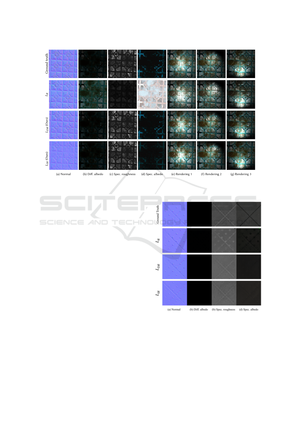
Figure 1: We overﬁt the model using the 3 different losses on renderings generated from the single property maps shown in

the ground truth row. Both the disentangled and integrated rendering loss predict maps extremely close to ground truth, while

traditional rendering loss predicts incorrect maps due to entanglement.

from both L

and L

show far more accurate re-

covery of SVBRDF maps. This can be credited to the

fact that when optimizing these new losses, the search

would consistently move in a direction that would im-

prove both the individual maps and their renderings.

4.3 Map Recovery

To reiterate, SVBRDF property maps recovered with

the earlier deﬁned rendering loss are very different

from ground truth because the focus is on creating

similar renders to the input images, without any re-

gard to the accuracy of individual maps. Figure 2.

shows some examples wherein using rendering loss

recovers inaccurate maps, whereas training with dis-

entangled render loss or integrated loss recovers more

accurate maps.

5 CONCLUSIONS, LIMITATIONS

AND FUTURE WORK

In this work we have addressed the problem of re-

covering more accurate, disentangled material prop-

erty maps from images. We deﬁne two versions of

a new loss function, the disentangled rendering loss

and the integrated rendering loss, to train a network.

Figure 2: Example of material property map recovery of

models trained with different losses.

By separating out the rendering of maps and analyti-

cally integrating the specular albedo term of the ren-

dering equation, we are able to recover more accurate

SVBRDF maps than before. Our solutions are unique

and require less computational resources while still

Disentangled Rendering Loss for Supervised Material Property Recovery

117

producing better results than previous work without

any network modiﬁcations .

Through intentional overﬁtting of the same model

with each of the different losses, we show property

entanglement and inaccuracy in SVBRDF predictions

when using traditional rendering loss, emphasizing

the need for our kind of loss formulations in SVBRDF

recovery. However, more can be done to improve pre-

dictions further, such as exploring other network ar-

chitectures, implementing the use of appropriate pri-

ors, and to increase generalization capabilioty of the

model through further data augmentation.

6 BROADER IMPACT

While the work presented is speciﬁc to material prop-

erties, such entanglement of component parameters

would be present in other areas of deep learning

research focused on recovering many parameters at

once. Transferring our strategy of deﬁning a dis-

entangled loss function by selectively learning these

parameters could potentially be transferred to these

problems. Thus the broader impact of this work can

be stated as follows:

1. Potential for this methodology of deﬁning a dis-

entangled loss function to be applied to analogous

problems.

2. Potential for this methodology of computing the

expectation of a stochastic loss function with re-

spect to some external parameters, as opposed to

Monte Carlo sampling those parameters to be ap-

plied to analogous problems.

3. More accurate material property recovery will re-

sult in more correct results for downstream appli-

cations like material matching, SVBRDF editing,

and AR/VR environments.

REFERENCES

Abadi, M., Barham, P., Chen, J., Chen, Z., Davis, A.,

Dean, J., Devin, M., Ghemawat, S., Irving, G., Isard,

M., et al. (2016). Tensorﬂow: A system for large-

scale machine learning. In 12th {USENIX} Sympo-

sium on Operating Systems Design and Implementa-

tion ({OSDI} 16), pages 265–283.

Aittala, M., Aila, T., and Lehtinen, J. (2016). Reﬂectance

modeling by neural texture synthesis. ACM Trans.

Graph., 35(4).

Ben-Artzi, A., Overbeck, R. S., and Ramamoorthi, R.

(2006). Real-time BRDF editing in complex lighting.

ACM Trans. Graph., 25(3):945–954.

Chen, M., Tang, Q., Wiseman, S., and Gimpel, K. (2019). A

multi-task approach for disentangling syntax and se-

mantics in sentence representations. arXiv preprint

arXiv:1904.01173.

Denton, E. L. et al. (2017). Unsupervised learning of dis-

entangled representations from video. In Advances in

neural information processing systems, pages 4414–

4423.

Deschaintre, V., Aittala, M., Durand, F., Drettakis, G., and

Bousseau, A. (2018). Single-image svbrdf capture

with a rendering-aware deep network. ACM Trans-

actions on Graphics (TOG), 37(4):128.

Deschaintre, V., Aittala, M., Durand, F., Drettakis, G., and

Bousseau, A. (2019). Flexible svbrdf capture with a

multi-image deep network. In Computer Graphics Fo-

rum, volume 38, pages 1–13. Wiley Online Library.

Dong, Y. (2019). Deep appearance modeling: A survey.

Visual Informatics, 3(2):59 – 68.

Gao, D., Li, X., Dong, Y., Peers, P., Xu, K., and Tong,

X. (2019). Deep inverse rendering for high-resolution

svbrdf estimation from an arbitrary number of images.

ACM Transactions on Graphics (TOG), 38(4):134.

Guarnera, G. C., Ghosh, A., Hall, I., Glencross, M., and

Guarnera, D. (2017). Material capture and representa-

tion with applications in virtual reality. In ACM SIG-

GRAPH 2017 Courses, SIGGRAPH ’17, New York,

NY, USA. Association for Computing Machinery.

Guo, J., Guo, Y., Pan, J., and Lu, W. (2018). Brdf analysis

with directional statistics and its applications. IEEE

transactions on visualization and computer graphics,

PP.

Hsieh, J.-T., Liu, B., Huang, D.-A., Fei-Fei, L. F., and

Niebles, J. C. (2018). Learning to decompose and

disentangle representations for video prediction. In

Advances in Neural Information Processing Systems,

pages 517–526.

uhtreiber, P., Knecht, M., and Traxler, C. (2011). Brdf

approximation and estimation for augmented reality.

In 15th International Conference on System Theory,

Control and Computing, pages 1–6.

Kingma, D. P. and Ba, J. (2014). Adam: A

method for stochastic optimization. arXiv preprint

arXiv:1412.6980.

Kurt, M. and Edwards, D. (2009). A survey of brdf models

for computer graphics. 10.1145/1629216.1629222,

ACM SIGGRAPH Computer Graphics.

Li, X., Dong, Y., Peers, P., and Tong, X. (2017). Model-

ing surface appearance from a single photograph using

self-augmented convolutional neural networks. ACM

Trans. Graph., 36(4).

Li, Z., Sunkavalli, K., and Chandraker, M. (2018a). Mate-

rials for masses: Svbrdf acquisition with a single mo-

bile phone image. In Ferrari, V., Hebert, M., Smin-

chisescu, C., and Weiss, Y., editors, Computer Vision

– ECCV 2018, pages 74–90, Cham. Springer Interna-

tional Publishing.

Li, Z., Xu, Z., Ramamoorthi, R., Sunkavalli, K., and Chan-

draker, M. (2018b). Learning to reconstruct shape

and spatially-varying reﬂectance from a single image.

ACM Trans. Graph., 37(6).

GRAPP 2021 - 16th International Conference on Computer Graphics Theory and Applications

118

Liu, X., Kumar, B. V., Jia, P., and You, J. (2019). Hard nega-

tive generation for identity-disentangled facial expres-

sion recognition. Pattern Recognition, 88:1–12.

Lu, B., Chen, J.-C., and Chellappa, R. (2019). Unsu-

pervised domain-speciﬁc deblurring via disentangled

representations. In Proceedings of the IEEE Confer-

ence on Computer Vision and Pattern Recognition,

pages 10225–10234.

Ronneberger, O., Fischer, P., and Brox, T. (2015). U-net:

Convolutional networks for biomedical image seg-

mentation. In International Conference on Medical

image computing and computer-assisted intervention,

pages 234–241. Springer.

Saryazdi, S., Murphy, C., and Mudur, S. (2020). The Prob-

lem of Entangled Material Properties in SVBRDF Re-

covery. In Klein, R. and Rushmeier, H., editors, Work-

shop on Material Appearance Modeling. The Euro-

graphics Association.

Schlick, C. (1994). An inexpensive brdf model for

physically-based rendering. Computer Graphics Fo-

rum, 13(3):233–246.

Shu, Z., Yumer, E., Hadap, S., Sunkavalli, K., Shecht-

man, E., and Samaras, D. (2017). Neural face editing

with intrinsic image disentangling. In Proceedings of

the IEEE Conference on Computer Vision and Pattern

Recognition, pages 5541–5550.

Smith, B. (1967). Geometrical shadowing of a random

rough surface. IEEE Transactions on Antennas and

Propagation, 15(5):668–671.

Walter, B., Marschner, S., Li, H., and Torrance, K. (2007).

Microfacet models for refraction through rough sur-

faces. pages 195–206.

APPENDIX

Network Architecture

The primary goal of our experiments is to show that

changing the loss function to our disentangled render-

ing loss enables us to recover more accurate material

property maps. Hence we wish to emphasize that we

have not deviated from state of the art work in terms

of architecture, training/test data, and training cycles.

To evaluate our disentangled rendering loss, we

adopt the state-of-the-art multi-image SVBRDF re-

covery network proposed by (Deschaintre et al.,

2019). We use the popular U-Net encoder-decoder

architecture (Ronneberger et al., 2015) in parallel to a

fully-connected track which transmits global informa-

tion in the network, shown in Figure 3. This network

then outputs 64 channels of feature maps for each in-

put image view with the same spatial dimensions as

the input. We then aggregate these feature maps by

using max pooling so that we will have 64 channels of

features of the same spatial dimensions as the input.

As is the case in (Deschaintre et al., 2019), we use

the max-pooling operator which enables our model to

handle any arbitrary number of views as inputs. Fi-

nally, the features are fed into 3 layers of convolutions

with non-linearities to output the 4 material property

maps.

Implementation Details

Training. We train our model for 300K iterations

using the Adam optimizer (Kingma and Ba, 2014)

with a learning rate of 2e-5. We use a batch size of 2

and the number of views for each input sample during

training is randomly chosen between 1 and 5. Train-

ing took 3 days on an Nvidia GTX 1080 Ti.

Dataset. We use the publicly available dataset

proposed by (Deschaintre et al., 2019)

. This dataset

contains 1,850 property maps of common material

types such as wood, metal, leather, plastic, etc. Dur-

ing training, input property maps are rendered in Ten-

sorﬂow (Abadi et al., 2016) with a randomly chosen

light and view direction, and then fed to the network.

Data augmentation. We use data augmentation to

make our trained network more generalized. We use

the same randomized linear interpolation of material

property maps as done by (Deschaintre et al., 2019),

which was shown to greatly improve accuracy.

Integrated Loss

Rendering Equation

The rendering equation is composed of a specular

term ( f

) and a diffuse term ( f

N,D,R,S

(

l,~v) = f

(

N,S,R,

l,~v) + f

(D) (4)

Where R

N,D,R,S

(

l,~v) is the rendering function under

some light direction

l and view direction ~v parame-

terized by the 4 material maps N, D, R and S which

are the normal, diffuse albedo, specular roughness

and specular albedo maps respectively. The Cook-

Torrance microfacet specular BRDF is expressed as:

(

N,S, R,

l,~v,

h) =

F(S,~v,

h)G(

N,R,~v,

l)D(

N,R,

N ·

l)(

N ·~v)

(5)

Where

h is the half vector, F(S,~v,

h) is the Fres-

nel function, G(

N,R,~v,

l) is the geometric shadowing

term, and D(

N,R,

h) is the Normal Distribution Func-

tion (NDF). For the Fresnel function F, we use an

https://repo-sam.inria.fr/fungraph/multi image

materials/supplemental multi images/materialsData multi

image.zip

Disentangled Rendering Loss for Supervised Material Property Recovery

119

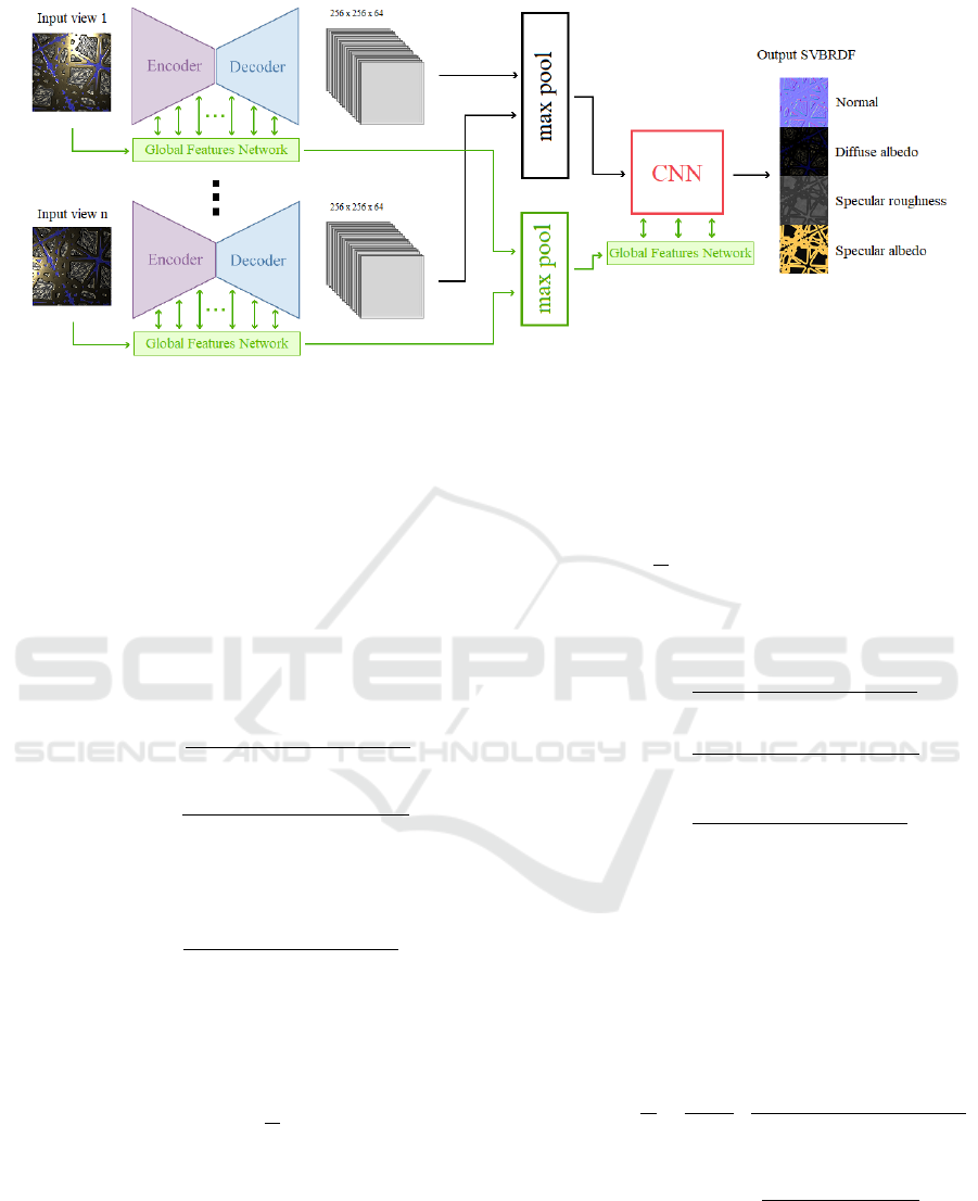
Figure 3: Network architecture.

approximation by Schlick(Schlick, 1994):

F(S,~v,

h) = S + (1 − S)2

−5.5(~v·

−6.98(~v·

(6)

For the geometric shadowing term G, we use Smith’s

method (Smith, 1967) which breaks G into light and

view components, and uses the same G

function for

both:

l,~v) = G

(

l)G

(~v) (7)

We use the Schlick-Beckmann approximation for G

(Schlick, 1994; Walter et al., 2007):

N,R,

l,~v) =

N ·

(

N ·

l)(1 − 0.5R

) + 0.5R

N ·~v

(

N ·~v)(1 − 0.5R

) + 0.5R

(8)

For the NDF term D, we use Trowbridge-Reitz GGX

(Walter et al., 2007):

N,R,

h) =

(

N ·

− 1) + 1

(9)

For the diffuse term, we assume a uniform diffuse

response over the microfacets hemisphere and use a

simple Lambertian model:

(D) =

(10)

Putting the above formulations together, our ﬁnal ren-

dering equation is:

N,D,R,S

(

l,~v) = f

(D) + f

(

N,S, R,

l,~v,

+ 0.25



S + (1 − S)2

−5.5(~v·

−6.98(~v·



(

N ·

l)(1 − 0.5R

) + 0.5R

(

N ·~v)(1 − 0.5R

) + 0.5R

(

N ·

− 1) + 1

(11)

Solving the Integral

We start by making the simplifying assumption that

our light and view direction are the same for our

renderings (

l = ~v =

h). By creating a new variable

t =

N ·~v, the simpliﬁed rendering equation will be:

N,D,R,S

(t) ≈

0.25S



t(1 − 0.5R

) + 0.5R





− 1) + 1



(12)

The optimization goal is to minimize the L1 error be-

tween ground truth renderings (R

N,D,R,S

(t)) and pre-

diction renderings (R

(

t)) over a variety of light

GRAPP 2021 - 16th International Conference on Computer Graphics Theory and Applications

120

and view directions. If we sample inﬁnite light and

view directions, we are effectively looking to com-

pute E

(t,

t)]:

(t,

t)] (13)

(t) − R

(

t)| f (t,

t)dtd

t (14)

+ |R

N,D,

− R

| (15)

D,R,

(

t) − R

(

t)| f (

t)d

t (16)

R,S

(

t) − R

(

t)| f (

t)d

t (17)

We assume the distribution of the view direction such

that we have the marginal probability density func-

tions

t ∼ U(0,1). This assumes that our views are

being sampled from directions which have a positive

dot product with the ground truth normal. Since com-

puting the expectation on the error of the normal map

(Eq. (11)) is not straight forward, we use an L1 loss

on the normal map instead:

= |N −

N| (18)

|D −

(19)

D,R,

(

t) − R

(

t)|d

t (20)

R,S

(

t) − R

(

t)|d

t (21)

To simplify the integration of Eq. (17) and Eq.

(18), we take the error on the log of the specular term

instead. This will not change the optimal solution that

will minimize this loss:



log(



Bt + 1





+ 1



)

− log(



Bt + 1





+ 1



)



log(



Bt + 1





+ 1



)

− log(



Bt + 1





+ 1



)



(22)

where:











A =

0.25SR

π(0.5R

)

A =

B =

1 − 0.5R

0.5R

− 1,

B =

− 1

C = R

− 1,

C =

− 1

(23)

We simplify log(1 + x) to x in order to get a much

simpler solution to the integral, as a complex solu-

tion is less likely to be adopted by the community

and will require more computation. Moreover, since

lim

x→∞

∂log(x+1)

∂x

= 0, for large values of x we will

have a gradient vanishing problem, which would not

be the case when simplifying log(1 + x) to x. Thus,

Eq. (19) will be reduced to:



(

−

)t + (

− R



+ |log(S) − log(

S)|

(24)

To make the implementation of the solution simpler,

we use the upper bound of the error on Eq. (21):

−

| +

− R

| + |log(S) − log(

S)| (25)

Thus the upper bound on the integrated rendering loss

would be:

=|N −

N| +

|D −

+ 2|

−

− R

| + |log(S) − log(

S)|

(26)

Disentangled Rendering Loss for Supervised Material Property Recovery

121