Improving Classification of Malware Families using Learning a Distance
Metric
Martin Jure
ˇ
cek, Olha Jure
ˇ
ckov
´
a and R
´
obert L
´
orencz
Faculty of Information Technology, Czech Technical University in Prague, Czech Republic
Keywords:
Malware Family, PE File Format, Distance Metric Learning, Machine Learning.
Abstract:
The objective of malware family classification is to assign a tested sample to the correct malware family. This
paper concerns the application of selected state-of-the-art distance metric learning techniques to malware fam-
ilies classification. The goal of distance metric learning algorithms is to find the most appropriate distance
metric parameters concerning some optimization criteria. The distance metric learning algorithms considered
in our research learn from metadata, mostly contained in the headers of executable files in the PE file format.
Several experiments have been conducted on the dataset with 14,000 samples consisting of six prevalent mal-
ware families and benign files. The experimental results showed that the average precision and recall of the
k -Nearest Neighbors algorithm using the distance learned on training data were improved significantly com-
paring when the non-learned distance was used. The k -Nearest Neighbors classifier using the Mahalanobis
distance metric learned by the Metric Learning for Kernel Regression method achieved average precision and
recall, both of 97.04% compared to Random Forest with a 96.44% of average precision and 96.41% of average
recall, which achieved the best classification results among the state-of-the-art ML algorithms considered in
our experiments.
1 INTRODUCTION
A large number of new malicious samples are cre-
ated every day, which makes manual analysis imprac-
tical. The majority of these samples are generated by
malware generators, which need to input some pa-
rameters. These malware generators, together with
their particular settings, define corresponding mal-
ware families. Samples generated from the same ge-
nerator with a fixed setting (i.e., from the malware
family) may be potentially similar to each other and
different from samples belonging to other malware
families or benign files. This work focuses on lever-
aging these differences to distinguish between mal-
ware families. Note that samples from the same mal-
ware family, however, generated in a different time
period may be different from each other (Wadkar
et al., 2020).
Since the samples are usually obfuscated, it is dif-
ficult to classify new (previously unseen) samples into
the correct malware families. Moreover, there is no
known general similarity measure suitable for a fea-
ture set extracted from the PE file format to correctly
cluster all malware families. (Jure
ˇ
cek and L
´
orencz,
2018) presented distance metric specially designed
for the PE file format that can handle all data types
of features.
Our work focuses on the multiclass classification
problem where each malware family and benign files
have their own class. This multiclass classification
problem is more challenging than a binary classifica-
tion problem where the goal is to distinguish between
malicious and benign files. However, the results of
(Basole et al., 2020) may indicate that an increasing
number of families (from 2 to 20 families) drops an
average balanced accuracy slightly.
The practical use of distinguishing between mal-
ware families lies in helping malware analysts to deal
with a large number of samples. Due to a large num-
ber of malicious files that come to antivirus vendors,
there is a need to automatically categorize malware
into groups corresponding to malware families. Sam-
ples belonging to the same group are similar to each
other with respect to some similarity measure (deter-
mined by distance metric). These groups are then dis-
tributed to malware analysts and assuming that files
belonging to the same group have similar behavior, it
may help speed up the further analysis.
Usually, malware analysts are specialists for some
limited number of malware families. If we assume
Jure
ˇ
cek, M., Jure
ˇ
cková, O. and Lórencz, R.
Improving Classification of Malware Families using Learning a Distance Metric.
DOI: 10.5220/0010326306430652
In Proceedings of the 7th International Conference on Information Systems Security and Privacy (ICISSP 2021), pages 643-652
ISBN: 978-989-758-491-6
Copyright
c
 2021 by SCITEPRESS – Science and Technology Publications, Lda. All rights reserved
643

that samples were classified correctly and samples of
the same family are similar to each other and dissim-
ilar to the samples of other families, using our ap-
proach, the analysts can focus only on those samples
which belong to the malware families for which the
analysts are specialized.
Good similarity measure plays an important role
in the performance of distance-based classifiers, such
as k -Nearest Neighbors (KNN). The distance be-
tween two feature vectors having the same class la-
bel must be minimized while the distance between
two feature vectors of different classes must be max-
imized. This is the goal of distance metric learning
methods used to learn the parameters of distance met-
rics from training data. As a result, they can poten-
tially improve the performance of the classifiers.
In our experiments, we consider six malware
families, which is a relatively small number. An-
other limitation of our work lies in assuming that our
dataset is large enough for training distance metric
learning (DML) algorithms. However, in practice,
new families or new malware variants are continu-
ously emerging. Therefore the training set, at some
moment, may not contain enough samples of the de-
sired malware family to train some supervised learn-
ing classifier.
The contributions of this paper are as follows:
• We determined and described the list of 25 fea-
tures all extracted (except one, i.e., size of a file)
from the PE file format. For each feature from
a section header, we considered the order of the
section rather than the type of the section (such as
.text, .data, .rsrc, etc.). While the sections’ order
turns out to be important for malware detection,
this kind of information is often not mentioned in
research papers.
• Using three DML algorithms, LMNN, NCA, and
MLKR, we achieved significantly better multi-
class classification results than any state-of-the-
art ML algorithms considered in our experiments.
We provided practical information concerning
performance, computational time, and resource
usage.
• We showed that the DML-based methods might
improve multiclass classification results even
when standard methods such as feature selection
or algorithm tuning were already applied. As a
result, we suggest using DML algorithms as an
important preprocessing step.
The rest of the paper is organized as follows. In
Section 2, we review recent malware detection me-
thods based on machine learning focusing on the clas-
sification of malware families. In Section 3, we give
some theoretical background and discuss three dis-
tance metric learning techniques used in our experi-
ments. The experimental setup and results of feature
selection algorithms are presented in Section 4. Sec-
tion 5 describes DML-based experiments and results.
We summarize our research work in Section 6.
2 RELATED WORK
This section briefly reviews the previous research pa-
pers on malware family classification related to our
work.
In (Basole et al., 2020), the authors conducted ex-
periments based on byte n-gram features, and they
considered 20 malware families. A binary classi-
fication were performed on different levels. In the
first level, for each of 20 families, they performed bi-
nary classification for 1,000 malware samples from
one family and 1,000 benign samples. In the se-
cond level, the malware class consists of two malware
families; in the third level, the malware class consists
of three malware families, and so on up to level 20,
where the malware class contains all of the 20 mal-
ware families. The authors applied four state-of-the-
art machine learning algorithms: KNN, Support Vec-
tor Machines, Random Forest, and Multilayer Percep-
tron. The best classification results (balanced accu-
racy) was achieved using KNN and Random Forest,
over 90% (at level 20), while KNN achieves the most
consistent results.
A fully automated system for analysis, classifi-
cation, and clustering of malware samples was in-
troduced in (Mohaisen et al., 2015). This system is
called AMAL and it collects behavior-based artifacts
describing files, registry, and network communica-
tion, to create features that are then used for classifica-
tion and clustering of malware samples into families.
The authors achieved more than 99% of precision and
recall in classification and more than 98% of precision
and recall for unsupervised clustering.
In (Ahmadi et al., 2016), the authors proposed
a malware classification system using different mal-
ware characteristics to assign malware samples to the
most appropriate malware family. The system allows
the classification of obfuscated and packed malware
without doing any deobfuscation and unpacking pro-
cesses. High classification accuracy of 99.77% was
achieved on the publicly accessible Microsoft Mal-
ware Challenge dataset.
(Islam et al., 2013) presented a classification
method based on static (function length frequency and
printable sting) and dynamic (API function names
with API parameters) features that were integrated
ICISSP 2021 - 7th International Conference on Information Systems Security and Privacy
644

into one feature vector. The obtained results showed
that integrating features improved classification accu-
racy significantly. The highest weighted average ac-
curacy was achieved by the meta-Random Forest clas-
sifier.
Another malware family classification system
referred to as VILO is presented in (Lakhotia
et al., 2013). They used TFIDF-weighted opcode
mnemonic permutation features and achieved bet-
ween 0.14% and 5.42% fewer misclassifications u-
sing KNN classifier than does the usage of n-gram
features.
In the rest of this section, we survey some previ-
ous works on distance metric learning applied to the
problem of malware detection. There is only a cou-
ple of works that address this topic. (Jure
ˇ
cek and
L
´
orencz, 2020) deals with measure learning and its
application to malware detection. Particle swarm op-
timization (PSO) was used to find appropriate feature
weights for the heterogeneous distance function used
in the KNN classifier. Positions of particles in the ini-
tialization step of PSO were set according to the in-
formation gain computed in the feature selection step
rather than randomly. As a result, PSO was acceler-
ated, and better classification accuracy was achieved
using the weighted distance function.
Work (Kong and Yan, 2013) concerns with a mal-
ware detection method based on structural informa-
tion. The discriminant distance metric is learned to
cluster the malware samples belonging to the same
malware family.
3 BACKGROUND
Performance of some ML classifiers, such as KNN,
depends significantly on the distance metric used to
compute similarity measure between two samples.
These classifiers rely on the assumption that samples
belonging to the same class are close to each other
(with respect to the distance function), and they are
far from samples belonging to the different classes.
The DML algorithms were designed to improve
the performance of distance-based classifiers via
learning the distance metric. This section provides
background and a brief description of three state-of-
the-art distance metric learning algorithms, LMNN,
NCA, and MLKR, used in our experiments.
Euclidean distance is by far the most commonly
used distance metric. Let x and y be two n-
dimensional feature vectors. The weighted Euclidean
distance is defined as follows:
d
w
(x, y) =
s
n
∑
i=1
w
2
i
(x
i
− y
i
)
2
(1)
where w
i
is a weight (non-negative real number)
associated with the jth feature. The distance metric
learning problem for weighted Euclidean distance is
defined as finding (or learning) an appropriate weight
vector w = (w
1
, . . . , w
n
) using training data, with re-
spect to some optimization criterion, usually mini-
mizing error rate.
Several distance functions have been presented
(Wilson and Martinez, 1997). To improve classifi-
cation or clustering results, many weighting schemes
were designed. A review of feature weighting me-
thods for lazy learning algorithms was proposed in
(Wettschereck et al., 1997).
Mahalanobis distance for two n-dimensional fea-
ture vectors x and y is defined as
d
M
(x, y) =
q
(x − y)
>
M(x − y) (2)
where M is a positive semidefinite matrix. Maha-
lanobis distance can be considered as a generalization
of Euclidean distance, since if M is the identity ma-
trix, then d
M
in Eq. (2) is reduced to Euclidean dis-
tance. If M is diagonal, this corresponds to learning
the feature weights M
ii
= w
i
from Eq. (1) defined for
weighted Euclidean distance.
The goal of learning the Mahalanobis distance is
to find an appropriate matrix M with respect to some
optimization criterion. In the context of the KNN
classifier, the goal is to find a matrix M, which is es-
timated from the training set, which leads to the lo-
west error rate of the KNN classifier. Since a positive
semidefinite matrix M can always be decomposed as
M = L
>
L, distance metric learning problem can be
viewed as finding either M or L = M
1
2
. Mahalanobis
distance defined in Eq. (2) expressed in terms of the
matrix L is defined as
d
M
(x, y) = d
L
(x, y) = kL
>
(x − y)k
2
(3)
The matrix L can be used to projects the origi-
nal feature space into a new embedding feature space.
This projection is a linear transformation defined for
feature vector x as
x
0
= Lx (4)
Note that the Mahanalobis distance d
L
(x, y) for
two samples from the original feature space equals the
Euclidean distance d(x
0
, y
0
) =
q
(x
0
− y
0
)
>
(x
0
− y
0
)
Improving Classification of Malware Families using Learning a Distance Metric
645

in the space transformed by Eq. (4). This transfor-
mation is usefull since computation of Euclidean dis-
tance has lower time complexity than computation of
Mahalanobis distance.
In the rest of this paper, we will consider the
feature space as a real n-dimensional space R
n
. The
following subsections briefly describe three distance
metric learning methods that we used in our experi-
ments.
3.1 Large Margin Nearest Neighbor
Large Margin Nearest Neighbor (LMNN) (Wein-
berger et al., 2006) is one of the state-of-the-art
distance metric learning algorithms used to learn a
Mahalanobis distance metric for KNN classification.
LMNN consists of two steps. In the first step, for each
instance, x, a set of k nearest instances belonging to
the same class as x (referred to as target neighbors)
is identified. In the second step, we adapt the Maha-
lanobis distance with the goal that the target neighbors
are closer to x than instances from different classes
that are separated by a large margin.
The Mahalanobis distance metric is estimated by
solving a semidefinite programming problem defined
as:
min
L
∑
i, j: j→i

d
L
(x
i
, x
j
)
2
+
+ µ
∑
k:y
i
6=y
k
max

0, 1 + d
L
(x
i
, x
j
)
2
− d
L
(x
i
, x
k
)
2

(5)
The notation j → i refers that the sample x
j
is a
target neighbor of the sample x
i
, and y
i
denotes the
class of x
i
. The parameter µ defines a trade-off be-
tween the two objectives.
3.2 Neighborhood Component Analysis
(Goldberger et al., 2005) proposed the Neighborhood
Component Analysis (NCA), a distance metric lear-
ning algorithm specially designed to improve KNN
classification.
Let p
i j
be the probability that the sample x
i
is the
neighbor of the sample x
j
belonging to the same class
as x
i
. This probability is defined as:
p
i j
=
exp(−||Lx
i
− Lx
j
||
2
2
)
∑
l6=i
exp(−||Lx
i
− Lx
l
||
2
2
)
, p
ii
= 0 (6)
The goal of NCA is to find the matrix L that ma-
ximizes the sum of probabilities p
i
:
argmax
L
N−1
∑
i=0
∑
j: j6=i,y
j
=y
i
p
i j
(7)
The well-known gradient ascent algorithm is used
to solve this optimization problem. Note that both
LMNN and NCA algorithms do not make any as-
sumptions on the class distributions.
3.3 Metric Learning for Kernel
Regression
(Weinberger and Tesauro, 2007) proposed Metric
Learning for Kernel Regression (MLKR), which aims
at training a Mahalanobis matrix by minimizing the
error loss over the training samples:
L =
∑
i
(y
i
− ˆy
i
)
2
(8)
where the prediction class ˆy
i
is derived from ker-
nel regression by calculating a weighted average of
the training samples:
ˆy
i
=
∑
j6=i
y
j
K(x
i
, x
j
)
∑
j6=i
K(x
i
, x
j
)
(9)
MLKR can be applied to many types of kernel
functions K(x
i
, x
j
) and distance metrics d(x, y).
Note that the mentioned distance metric learning
algorithms can be used as supervised dimensionality
reduction algorithms. Considering the matrix L ∈
R
d×n
with d < n then the dimension of transformed
sample x
0
= Lx is reduced to d.
4 EXPERIMENTAL SETUP
In this section, we present our dataset, describe eval-
uation measures and feature selection results.
4.1 Dataset
Our experiments are based on the dataset contain-
ing 14,000 samples consisting of 6 malware families
and benign files. The dataset is well-balanced since
each of the 6 malware families is of equal size, i.e.,
2,000 samples, and the number of benign files is also
2,000. The malicious programs were obtained from
(VirusShare, 2020), an online repository containing
various malware families. Benign files were gathered
from university computers. We confirm that all mali-
cious samples considered in our experiments match
ICISSP 2021 - 7th International Conference on Information Systems Security and Privacy
646

known signatures from antivirus companies. Also,
none of our benign programs was detected as mal-
ware.
In our experiments, we used the following six
prevalent malware families:
Allaple – a polymorphic network worm that spreads
to other computers and performs denial-of-service
(DoS) attacks.
Skeeyah – a Trojan horse that infiltrates systems and
steals various personal information and adds the
computer to a botnet.
Virlock – ransomware that locks victims’ computer
and demands a payment to unlock it.
Virut – a virus with backdoor functionality that ope-
rates over an IRC-based communications proto-
col.
Vundo – a Trojan horse that displays pop-up adver-
tisements and also injects JavaScript into HTML
pages.
Zbot – also known as Zeus, is a Trojan horse that
steals configuration files, credentials, and banking
details.
4.2 Evaluation Measures
In this section, we present the metrics we used to mea-
sure the performance of the classification models. In a
binary classification problem, the following classical
quantities are employed:
• True Positive (TP) represents the number of mali-
cious samples classified as malware
• True Negative (TN) represents the number of be-
nign samples classified as benign
• False Positive (FP) represents the number of be-
nign samples classified as malware
• False Negative (FN) represents the number of ma-
licious samples classified as benign
The performance of binary classifiers considered
in our experiments is measured using three standard
metrics. The most intuitive and commonly used eval-
uation metric is the error rate:
ERR =
FP + FN
TP + TN + FP + FN
(10)
It is defined on a given test set as the percentage
of incorrectly classified samples. Alternative for error
rate is accuracy defined as ACC= 1−ERR. The se-
cond metric is precision, and it is defined as follows:
precision =
TP
TP + FP
(11)
Precision is the percentage of samples classified as
malware that are truly malware. The third parameter,
recall (or true positive rate), is defined as:
recall =
TP
TP + FN
(12)
Recall is the percentage of truly malicious sam-
ples that were classified as malware.
In the multiclass evaluation, since all the classes
have the same number of samples, we use averaged
versions of error rate, precision and recall. Average
error rate is defined as follows:
(average) ERR =
1
N
∑
i≤N
1
class
pred
6= class
true
(13)
where N is the size of our dataset, and 1 is the
indicator function. Average precision and average re-
call is defined as an average resulting precisions and
recalls, respectively, across all classes.
4.3 Feature Selection
The features used in our experiments are extracted
from the portable executable (PE) file format (Mi-
crosoft, 2019), which is the file format for executa-
bles, DLLs, object code, and others used in 32-bit and
64-bit versions of the Windows operating system. The
PE file format is the most widely used file format for
malware samples run on desktop platforms.
For extracting features from PE files, we used
Python module pefile (Carrera, 2017). This modu-
le extracts all PE file attributes into an object from
which they can be easily accessed. We extracted 358
numeric features that are based on static information
only, i.e., without running the program. The dimen-
sionality is high since for each section, and for each
kind of characteristics (array of flags), we consider
each flag as a single feature.
Before applying feature selection methods,
all features were normalized using procedure
preprocessing.normalize from the Scikit-learn
library (Scikit-learn, 2020). We then employed the
six feature selection methods also imported from the
Scikit-learn library.
Table 1 shows error rates of the KNN (k = 1) clas-
sifier applied to the feature set reduced using the cor-
responding feature selection algorithms. The lowest
error rate of 4.13% was achieved for 25 selected fea-
tures by RFE Logistic Regression. The KNN for the
original feature set (i.e., 358 features) achieved an er-
ror rate of 4.31%. All feature selection algorithms
were evaluated by 5-fold cross-validation on the ran-
domly chosen training data containing 80% of the
whole dataset. The remaining 20% of the dataset was
Improving Classification of Malware Families using Learning a Distance Metric
647

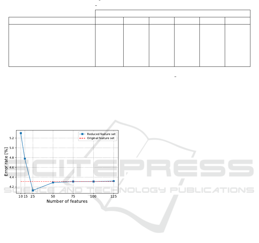
Table 1: Evaluation of the feature selection algorithms in terms of error rates of the KNN (k = 1) classifier. The abbreviation
SFM refers to Scikit-learn procedure feature selection.SelectFromModel. The abbreviation RFE refers to Recursive
Feature Elimination implemented in feature selection.RFE from the Scikit-learn library as well.
Error rates [%] for specific number of features
Feature selection method 2 5 10 25 50 75
Principal component analysis 11.00 5.30 4.85 4.22 4.26 4.31
SFM Logistic Regression 13.61 7.90 4.76 4.20 4.29 4.31
SFM Decision Tree 26.56 8.44 6.21 4.72 4.50 4.37
Information Gain 15.17 8.77 7.79 5.61 4.31 4.52
RFE Logistic Regression 17.08 6.49 5.30 4.13 4.29 4.31
RFE Decision Tree 11.67 7.53 4.76 4.63 4.65 4.22
reserved for testing the DML and ML algorithms (see
Section 5).
The following Fig. 1 illustrates the performance
of RFE Logistic regression for a various number of
features. For 50 and more features, the corresponding
error rates are approximately the same as the error
rate achieved from the original feature set (i.e., 358
features).
Figure 1: Relation between dimensionality and error rate of
KNN classifier (k = 1).
Notice that for each feature selection algorithm
under consideration, except SFM Decision Tree, we
achieved a surprisingly low error rate with only two
features, as shown in Table 1. We will provide more
experiments for this extremely low dimensionality in
Section 5.2.
We also performed all six feature selection algo-
rithms to explore an even higher number of features:
100, 125, and 150. However, the corresponding er-
ror rates achieved from all the feature selection algo-
rithms were higher than 4.13%. As a result, in all ex-
periments (except those in Section 5.2), we will con-
sider 25 features selected by RFE Logistic regression
algorithm. To make our results reproducible, Table 2
summarizes all features used in our experiments. We
keep the name of the fields in the same form as in
the documentation (Microsoft, 2015), in order that the
reader can easily find the detailed description.
The field file size (size of the file on disk) is not
contained within the PE structure, and note that it dif-
fers from the field SizeOfImage, which is the size of
the image loaded in memory.
PE files are divided into one or more sections. The
sections contain code, data, imports, and various cha-
racteristics. PE section features are considered sepa-
rately for each section. The order of the sections is
not the same for each PE file. Moreover, malware au-
thors can change the order of the sections. Therefore,
we prefer to consider only the order of sections (rather
than their names). The special importance among all
sections of a PE file has the last one since it may
contain useful information, especially for some types
of malware, such as file infector, which typically at-
taches malicious code at the end of the file. To deal
with a various number of sections across the samples,
we have decided to consider only the first four sec-
tions and the last section.
5 EXPERIMENTAL RESULTS
This section presents multiclass classification results
based on six base ML classifiers: k-Nearest Neigh-
bor (k = 1), Logistic Regression, (Gaussian) Naive
Bayes, Random Forest (number of trees in the for-
est = 100), and Multilayer Perceptron (hidden layer
sizes=(200,100), maximum number of iterations =
300, activation function = ’relu’, solver for weight op-
timization = ’adam’, random number generation for
weights and bias initialization = 1). Implementations
of the DML algorithms, the ML classifiers, and the
classification metrics, are based on the Scikit-learn
library (Scikit-learn, 2020). If not mentioned, the
hyperparameters of the ML classifiers and the DML
methods were set to their default values as set in the
Scikit-learn library.
The input feature vectors used in the following ex-
periments are described in Section 4.3, and its dimen-
sionality is 25, except in the experiment described in
Section 5.2 where we consider only two-dimensional
ICISSP 2021 - 7th International Conference on Information Systems Security and Privacy
648

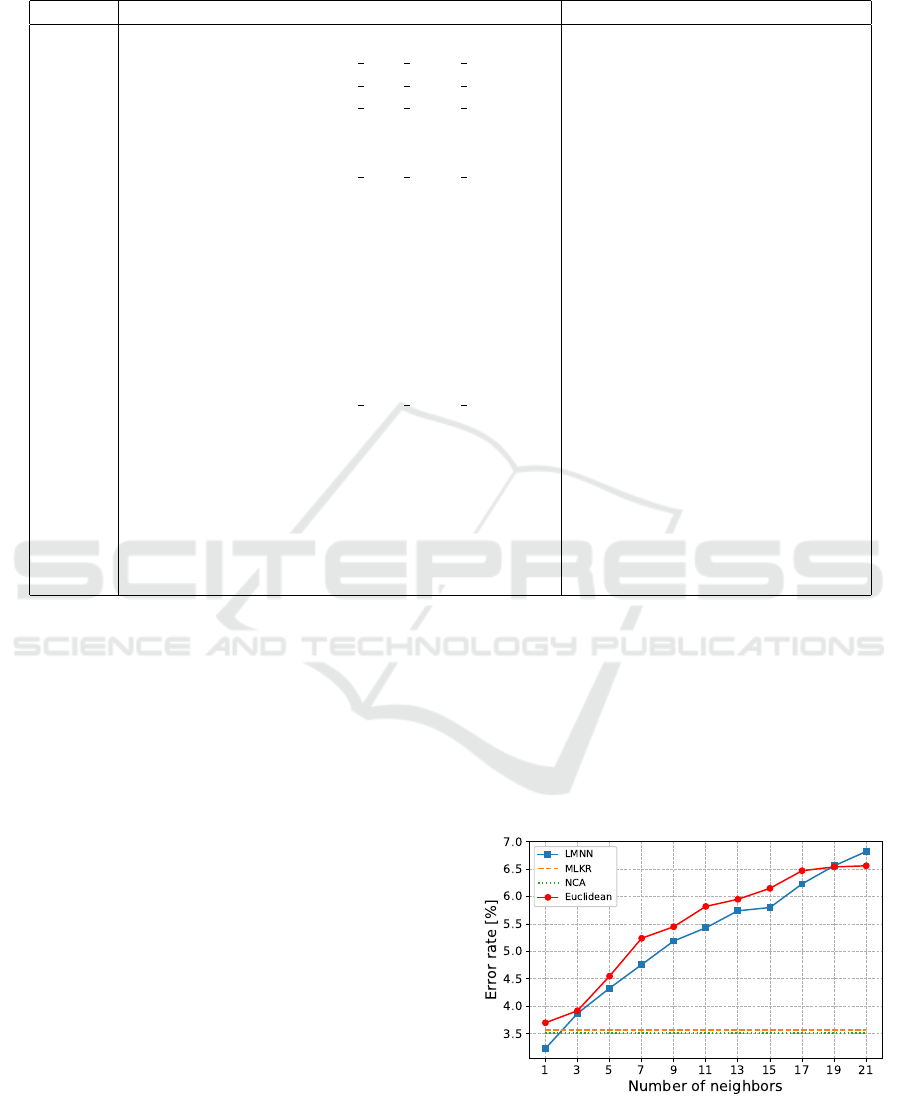
Table 2: List of 25 features selected by the RFE Logistic Regression algorithm sorted by importance. All except one (file
size) are extracted from the PE file format.
Position Feature name Structure
1. PointerToRawData Section Header (the first section)
2. Characteristics, flag IMAGE SCN TYPE DSECT Section Header (the first section)
3. Characteristics, flag IMAGE SCN TYPE COPY Section Header (the first section)
4. Characteristics, flag IMAGE SCN TYPE NOLOAD Section Header (the first section)
5. RVA of Exception Table Optional Header Data Directories
6. PointerToRawData Section Header (the third section)
7. Characteristics, flag IMAGE SCN TYPE GROUP Section Header (the first section)
8. RVA of Certificate Table Optional Header Data Directories
9. RVA of Base RelocationTable Optional Header Data Directories
10. RVA of Bound Import Optional Header Data Directories
11. VirtualSize Section Header (the first section)
12. SizeOfRawData Section Header (the first section)
13. Size of file not part of PE format
14. VirtualAddress Section Header (the fourth section)
15. VirtualSize Section Header (the second section)
16. RVA of Import Table Optional Header Data Directories
17. Characteristics, flag IMAGE SCN TYPE REG Section Header (the first section)
18. AddressOfEntryPoint Optional Header Standard Fields
19. RVA of Export Table Optional Header Data Directories
20. VirtualAddress Section Header (the first section)
21. RVA of TLS Table Optional Header Data Directories
22. PointerToRawData Section Header (the second section)
23. VirtualAddress Section Header (the last section)
24. Size of Import Table Optional Header Data Directories
25. VirtualAddress Section Header (the second section)
feature vector.
All the following experiments were executed on a
single computer platform having two processors (Intel
Xeon Gold 6136, 3.0GHz, 12 cores each), with 32
GB of RAM running the Ubuntu server 18.04 LTS
operating system.
5.1 Application of Distance Metric
Learning Algorithms
In the first set of experiments, we applied the
KNN classifier using the following four distances:
Euclidean (non-learned) distance, and three Maha-
lanobis distances learned by three DML algorithms
(separately) LMNN, NCA, and MLKR. We used 5-
fold cross-validation as follows. The training dataset
(80 % of the whole dataset) was randomly divided
into five subsets of equal size, where four subsets
were used for training the DML algorithms, and one
subset was used for testing. First, the DML algorithm
was trained on the four subsets, and then KNN with
learned Mahalanobis distance metric was employed
using training and testing sets. This procedure was
run five times with different subset reserved for tes-
ting. Classification results obtained for each fold are
then averaged to produce a single cross-validation es-
timate.
The first experiment focuses on the hyperpara-
meter k that expresses the number of nearest neigh-
bors considered in the KNN classifier and LMNN (the
learning rate of the optimization procedure = 10
−6
)
algorithm. Note that both MLKR nor NCA do not de-
pend on k. Fig. 2 shows the effect of k on the error
rate of the KNN using all four distances.
Figure 2: The relation between the number of nearest neigh-
bors (k) and error rate (ERR) compared for four distances.
Improving Classification of Malware Families using Learning a Distance Metric
649

The KNN classifier for k = 1 with Euclidean dis-
tance achieved the ERR of 3.70%. Error rates of the
KNN using Mahalanobis distance learned by DML al-
gorithms are equal to: 3.23% for LMNN, 3.51% for
NCA, and 3.57% for MLKR.
The result of distance metric learning algorithms
is n×n matrix, where n is the dimension of the feature
vector. Since the number of components of the matrix
to be learned grows at a quadratic rate and the size of
the training data is fixed, we can expect that the size of
training data stops being sufficient for high values of
n. In the next experiment, we used the Principal com-
ponent analysis to reduce the data’s dimension and
examine the learning ability of distance metric learn-
ing algorithms. We applied 5-fold cross-validation
technique described above. For our fixed-size training
dataset, the highest performance improvement gained
by using DML algorithms was achieved for the fol-
lowing dimensions: n = 3 for LMNN, n = 4 for NCA,
and n = 6 for MLKR. These results may indicate that
considering 25-dimensional feature vectors used in
our experiments, our dataset’s size is insufficient for
learning as many as 625 parameters (i.e., the number
of components of the matrix M).
We also explored the variation of classification re-
sults based on DML algorithms across six malware
families and benign class. Precisions and recalls of
the KNN classifier using the hyperparameter k = 1
are summarize in Table 3. The results indicate that
the precisions and recalls corresponding to malware
families depend significantly on the DML algorithms.
Regarding resource usage of DML algorithms,
32GB of RAM was sufficiently enough (i.e., with-
out a need to use the disk as swap memory) for all
conducted experiments. The average computational
times of the DML algorithms applied on 8,960 sam-
ples are as follows: LMNN took 550 seconds, NCA
took 960 seconds, and MLKR took 4, 800 seconds.
5.2 Representation of Malware Families
in Two Dimensions
In this section, we examine the classification results
based on two-dimensional feature vectors. Two of the
most important features, PointerToRawData and flag
IMAGE SCN TYPE DSECT (see Table 2), were se-
lected by the RFE Logistic Regression and used for
multiclass classification.
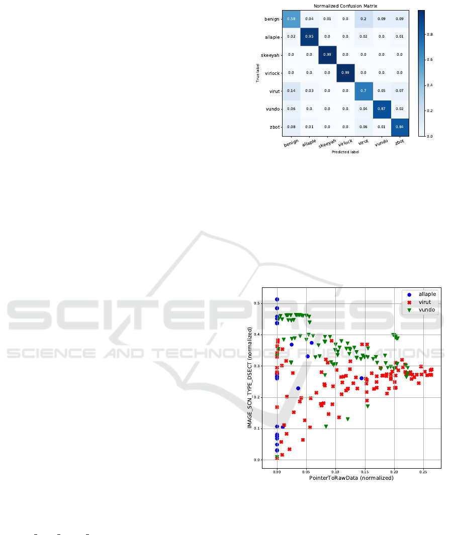
Fig. 3 presents the effectiveness of the KNN (k =
1) classification of malware families and benign files
represented by only two-dimensional feature vectors.
While we achieved 99% accuracy for the malware
families Skeeyah and Virlock, benign files’ accuracy
was 58%.
Figure 3: Normalized confusion matrix comparing the ac-
curacy of KNN (k = 1) using Euclidean distance for six mal-
ware families and benign samples.
Two-dimensional representation of feature vectors
allows us to show malware families as points in the
plane. Three malware families, Allaple, Virut, and
Vundo, are illustrated in Fig. 4. One hundred samples
were chosen randomly from each of these classes,
and we achieved the average classification accuracy
of 92.00%.
Figure 4: Three malware families: Allaple, Virut, and
Vundo represented in two dimensions.
5.3 Comparison with the
State-of-the-Art ML Algorithms
In the last experiment, LMNN, NCA, and MLKR
methods (each separately) were used to transform the
data, as it is shown in Eq. (4) in Section 3. We com-
pared the performance of the state-of-the-art ML al-
gorithms for original (non-transformed) data and for
the transformed data. Table 4 shows that the high-
ICISSP 2021 - 7th International Conference on Information Systems Security and Privacy
650

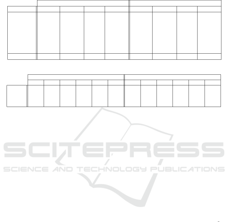
Table 3: KNN (k = 1) classification results of particular malware families and class of benign samples.
Precision [%] Recall [%]
class Euclid LMNN NCA MLKR Euclid LMNN NCA MLKR
allaple 98.58 98.79 92.32 92.39 98.42 98.49 92.60 91.69
benign 94.48 94.24 99.24 99.09 92.08 92.15 97.47 97.47
skeeyah 99.36 98.45 98.88 98.41 98.89 98.30 99.04 99.04
virlock 98.79 99.55 99.72 100 99.39 99.40 99.15 99.15
virut 97.24 96.51 97.38 96.19 95.44 97.07 96.49 96.49
vundo 95.38 97.26 94.85 95.27 98.07 97.71 98.43 98.11
zbot 92.65 92.59 93.03 93.50 94.21 94.34 92.33 93.08
Averaged 96.64 96.77 96.49 96.41 96.64 96.78 96.50 96.43
Table 4: Classification results of DML algorithms evaluated for several state-of-the-art ML algorithms.
Average precision [%] Average recall [%]
KNN LR NB DT RF MLP KNN LR NB DT RF MLP
original 96.15 86.38 82.98 94.76 96.44 96.22 96.14 86.17 77.79 94.78 96.41 96.17
LMNN 96.77 89.55 82.02 95.20 97.05 96.39 96.78 89.27 81.03 95.20 97.00 96.35
NCA 96.45 90.78 78.08 94.87 96.76 95.11 96.46 90.60 75.02 94.86 96.72 95.07
MLKR 97.04 87.94 77.96 95.15 97.05 96.50 97.04 88.12 75.41 95.13 97.02 96.49
est average precision of 97.05% was achieved using
Random Forest on the data transformed by LMNN or
by MLKR. The KNN classifier achieved the highest
average recall of 97.04% on the data transformed by
MLKR.
Regarding original (non-transformed) data, the
highest average precision of 96.44% and the highest
average recall of 96.41% among base ML algorithms
were both achieved by Random Forest.
Focusing on the KNN (k = 1) classifier, any of
the three DML methods achieved better classifica-
tion results (both average precision and recall) than
the KNN classifier using common (non-learned) Eu-
clidean distance. Regarding the Naive Bayes classi-
fier, we achieved a very low precision of 54.53% for
Vundo and a very low recall of 47.02% for Zbot com-
pared to other ML classifiers. These two results cause
that average precision and recall for Naive Bayes are
significantly lower compared to other ML algorithms.
6 CONCLUSIONS
In this paper, we employed three distance metric
learning algorithms to learn the Mahalanobis dis-
tance metric to improve multiclass classification per-
formance for our dataset containing six prevalent mal-
ware families and benign files. We classified the
previously unseen samples using the KNN classifier
with the learned distance and achieved significantly
better results than using common (non-learned) Eu-
clidean distance. The classification results demon-
strate that DML-based methods outperform any of the
state-of-the-art ML algorithms considered in our ex-
periments. Our results indicate that the classification
performance based on DML methods could be further
improved if we use a larger dataset for training the
distance metric. Another experiment was concerned
with low-dimensional representations of the input fea-
ture space. We achieved surprisingly good classifica-
tion results even for two-dimensional feature vectors.
In future work, other types of features, such as
byte sequences, opcodes, API and system calls, and
others, could be used and possibly improve the classi-
fication results. It would also be interesting to explore
the application of distance metric learning algorithms
to clustering into malware families.
ACKNOWLEDGEMENTS
The authors acknowledge the support of the OP VVV
MEYS funded project CZ.02.1.01/0.0/0.0/16 019/
0000765 ”Research Center for Informatics”.
REFERENCES
Ahmadi, M., Ulyanov, D., Semenov, S., Trofimov, M., and
Giacinto, G. (2016). Novel feature extraction, selec-
tion and fusion for effective malware family classifi-
cation. In Proceedings of the sixth ACM conference
on data and application security and privacy, pages
183–194.
Basole, S., Di Troia, F., and Stamp, M. (2020). Multifamily
malware models. Journal of Computer Virology and
Hacking Techniques, pages 1–14.
Carrera, E. (2017). Pefile. https://github.com/erocarrera/
pefile.
Improving Classification of Malware Families using Learning a Distance Metric
651

Goldberger, J., Hinton, G. E., Roweis, S. T., and Salakhutdi-
nov, R. R. (2005). Neighbourhood components anal-
ysis. In Advances in neural information processing
systems, pages 513–520.
Islam, R., Tian, R., Batten, L. M., and Versteeg, S. (2013).
Classification of malware based on integrated static
and dynamic features. Journal of Network and Com-
puter Applications, 36(2):646–656.
Jure
ˇ
cek, M. and L
´
orencz, R. (2018). Malware detection
using a heterogeneous distance function. Computing
and Informatics, 37(3):759–780.
Jure
ˇ
cek, M. and L
´
orencz, R. (2020). Distance metric
learning using particle swarm optimization to improve
static malware detection. In Int. Conf. on Information
Systems Security and Privacy (ICISSP), pages 725–
732.
Kong, D. and Yan, G. (2013). Discriminant malware dis-
tance learning on structural information for automated
malware classification. In Proceedings of the 19th
ACM SIGKDD international conference on Knowl-
edge discovery and data mining, pages 1357–1365.
ACM.
Lakhotia, A., Walenstein, A., Miles, C., and Singh, A.
(2013). Vilo: a rapid learning nearest-neighbor classi-
fier for malware triage. Journal of Computer Virology
and Hacking Techniques, 9(3):109–123.
Microsoft (2019). Pe format - win32 apps.
https://docs.microsoft.com/en-us/windows/win32/
debug/pe-format.
Microsoft (Revision 9.3, 2015). Visual studio, microsoft
portable executable and common object file format
specification.
Mohaisen, A., Alrawi, O., and Mohaisen, M. (2015).
Amal: High-fidelity, behavior-based automated mal-
ware analysis and classification. computers & secu-
rity, 52:251–266.
Scikit-learn (2020). scikit-learn.org. https://scikit-learn.
org/.
VirusShare (2020). Virusshare.com. http://virusshare.com/.
Wadkar, M., Di Troia, F., and Stamp, M. (2020). Detect-
ing malware evolution using support vector machines.
Expert Systems with Applications, 143:113022.
Weinberger, K. Q., Blitzer, J., and Saul, L. K. (2006). Dis-
tance metric learning for large margin nearest neigh-
bor classification. In Advances in neural information
processing systems, pages 1473–1480.
Weinberger, K. Q. and Tesauro, G. (2007). Metric learn-
ing for kernel regression. In Artificial Intelligence and
Statistics, pages 612–619.
Wettschereck, D., Aha, D. W., and Mohri, T. (1997). A
review and empirical evaluation of feature weighting
methods for a class of lazy learning algorithms. Arti-
ficial Intelligence Review, 11(1-5):273–314.
Wilson, D. R. and Martinez, T. R. (1997). Improved het-
erogeneous distance functions. Journal of artificial
intelligence research, 6:1–34.
ICISSP 2021 - 7th International Conference on Information Systems Security and Privacy
652