Segmentation of Agricultural Images using Vegetation Indices

Jean Fabr

ıcio Batista Santos, Jocival Dantas Dias Junior, Andr

e Ricardo Backes

and Maur

ıcio Cunha Escarpinati

School of Computer Science, Federal University of Uberl

andia, Brazil

Keywords:

Precision Agriculture, Plant Segmentation, Vegetation Indices.

Abstract:

Identifying and segmenting plants from the background in agricultural images is of great importance for pre-

cision agriculture. It serves as a basis for several tasks such as identiﬁcation of planting lines, identiﬁcation

of weed plants, agricultural automation, among others. Given this importance, in this paper, we evaluated

the application of ﬁve vegetation indices for RGB images together with two binarization techniques for the

plant/background segmentation process. The results showed promising performance in all evaluated indices.

It was also possible to identify a relationship between the performance obtained in each index and the capture

conditions in each dataset.

1 INTRODUCTION

The diversity of land areas, types of soils and plants,

products, and machinery makes the management of

a simple planting area a complex task. To facilitate

this task, in the last few decades Precision Agricul-

ture (PA) has emerged as a new way to manage agri-

cultural resources. Literature deﬁnes PA as the use of

different technologies (such as artiﬁcial intelligence,

internet of things, data analysis, and image process-

ing) with the main objective of optimizing results, re-

ducing costs, and creating a more sustainable produc-

tion chain.

A simple example of PA applied to a plantation

is the use of an Unmanned Aerial Vehicle (UAV) to

acquire images of the plantation. Depending on the

sensors present in the UAV, it is possible to obtain a

map of the area with many types of information, such

as land topology and vegetation distribution. There is

a wide range of sensors that can be used with a UAV.

The most common are cameras that capture color pat-

terns in RGB format. However, other bands, such as

infrared and ultraviolet, can be also used. RGB cam-

eras are widely used in image processing because they

are the standard that most devices use, such as smart-

phones, allowing image processing algorithms to run

even in mobile applications (Riehle et al., 2020). By

using speciﬁc algorithms, it is possible to extract from

these maps high-level information from the area, such

as the location of crop lines, plant count, and the pres-

ence of sowing failures. These informations enable

the farm to improve the use of the resources and al-

lows the use of other operations such as robots, trac-

tors, and autonomous pruning (Bargoti and Under-

wood, 2016).

Identifying and separating plants from the soil is

an important task because it allows the monitoring of

plant growth, health, and the identiﬁcation of pests

and weeds. Mathematical equations applied to the

RGB channels of the images result in different in-

dices that highlight certain wavelengths, such as the

green levels of the image, thus facilitating the sep-

aration of the plant from background pixels (Riehle

et al., 2020). However, an index that highlights green

pixels is not enough to separate weed crops, and other

types of vegetation index may be needed for this prob-

lem. The use of vegetation indices has some advan-

tages such as low computational cost in comparison

with other segmentation techniques or machine learn-

ing approaches, easy implementation, and handling.

Nevertheless, they are sensitive to brightness varia-

tion, presence of shadows, and manual deﬁnition of

the threshold (Riehle et al., 2020).

In literature, there are a wide variety of RGB in-

dices that can be used for image segmentation pur-

poses. In the present work, we aimed to evaluate some

of these vegetation indices in a plant/soil segmenta-

tion task when combined with a clustering algorithm

and a simple threshold method to obtain the differ-

ent regions of interest. We compared the performance

of each vegetation index in the dataset presented in

(Riehle et al., 2020), which presents images with pre-

deﬁned masks of the plant/soil regions.

The remaining of the paper is structured as fol-

506

Santos, J., Dias Junior, J., Backes, A. and Escarpinati, M.

Segmentation of Agricultural Images using Vegetation Indices.

DOI: 10.5220/0010325005060511

In Proceedings of the 16th International Joint Conference on Computer Vision, Imaging and Computer Graphics Theory and Applications (VISIGRAPP 2021) - Volume 4: VISAPP, pages

506-511

ISBN: 978-989-758-488-6

lows: Section 2 presents a review of recent paper pub-

lished on this topic and that motivated our research.

In Section 3 we describe the vegetation indices used

in this work as also the datasets used for evaluation.

Section 4 describes how experiments were performed

while Section 5 presents the results obtained by each

vegetation index. Finally, Section 6 concludes the pa-

per.

2 RELATED WORK

Computing a vegetation index is a common pre-

processing technique used for plant/soil segmentation

problems. It increases the contrast between vegeta-

tion and soil, generating a grayscale image that high-

lights particular regions of interest. For example, the

Excess Green Index (ExG) and the Excess Red Index

(ExR) aim to increase the contract of the Green and

Red levels, respectively, highlighting the plant from

other elements, such as soil and waste. And when

combined, these indices can generate even more efﬁ-

cient results in segmentation, such as ExGR (Riehle

et al., 2020), which is calculated as follows:

ExG = 2G − R − B (1)

ExR = 1.4R − B (2)

ExGR = ExG − ExR (3)

ExGR index results in an image where pixels

range from positive (plant) to negative (soil and

residues) values so that the image is easily segmented

using a ﬁxed threshold at zero value, without the need

to use an automatic threshold method, such as Otsu

(Otsu, 1979).

Another way to use these indices is to generate

masks from the indexed image. While the ExG index

highlights the pixels of the green channel of the im-

age, the ExR index highlights the red channel. These

two indices can be used to produce a mask for, re-

spectively, vegetation and background, that combined

by a logical AND operation enable us to extract the

vegetation of the original image (Riehle et al., 2020).

Other methods can be used to segment

plant/background without the need for manual

parameterization (e.g., threshold or color selection).

Some approaches use Naive Bayes to classify the

pixels belonging to the plant and background (Abbasi

and Fahlgren, 2016). First, the image is converted

from RGB to HSV color model. Then, the color

distribution of vegetation and soil are approximated

by probability distribution functions, which allows

the use of the Naive Bayes method to segment the

plants.

More recently, deep learning approaches, such

as Deep Convolutional Neural Networks (DCNN’s),

have been proposed as an alternative for plant/soil

segmentation problems. This is explained due to their

great success in many classiﬁcation and segmentation

problems in different areas. They have been proven to

be very efﬁcient in identifying objects and as a generic

solution for various types of soils, terrains, and ex-

posure to sunlight and shading. The network archi-

tecture varies from problem to problem as, for exam-

ple, the number of convolutional and pooling layers

(Zhuang et al., 2018). Depending on the application,

the input can be images generated from the vegetation

indices or simple RGB images. Performance analy-

sis, however, shows that vegetation indices generate

information loss and that using RGB images as input

usually generates better results (Zhuang et al., 2018).

For segmentation purposes, the basic structure of a

DCNN is composed of an encoder and a decoder. The

encoder is trained to compress and to extract image

features by using several convolutional layers, orga-

nized hierarchically, where each layer corresponds to

a different semantic level. In the sequence, the de-

coder reconstructs the input image based on the model

compressed by the encoder, thus resulting in an image

labeled with different regions of interest.

3 MATERIALS AND METHODS

3.1 Vegetation Indices

Given its usage in several precision agriculture works,

we evaluated the following plant/background indices

for segmentation: Modiﬁed Green Red Vegetation

(4) (Bendig et al., 2015), Green Leaf Index (Equa-

tion 5) (Louhaichi et al., 2001), Modiﬁed Photo-

chemical Reﬂectance Index (Equation 6) (Yang et al.,

2018), Red Green Blue Vegetation Index (Equation 7)

(Bendig et al., 2015), Excess of Green (Equation 8)

(Woebbecke et al., 1995) and Vegetativen (Equation

9) (Hague et al., 2006):

MGRV =

− R

+ R

(4)

GLI =

2G − R − B

2G + R + B

(5)

MPRI =

G − R

G + R

(6)

RGBV I =

G − (B ∗ R)

) + (B ∗ R)

(7)

Segmentation of Agricultural Images using Vegetation Indices

507

ExG = 2G − R − B (8)

V EG =

∗ B

(9)

* a = 0.667 and b = (1-a)

While ExG, GLI and VEG highlight pixels in the

green channel, MGRVI, MPRI, and RGBVI highlight

more than one channel of the image. For example,

MGRVI enhances the information of both green and

red channels, while MPRI emphasizes the reﬂectance

produced by chlorophyll present in leaves. These in-

dices act directly with the ability of the soil and plants

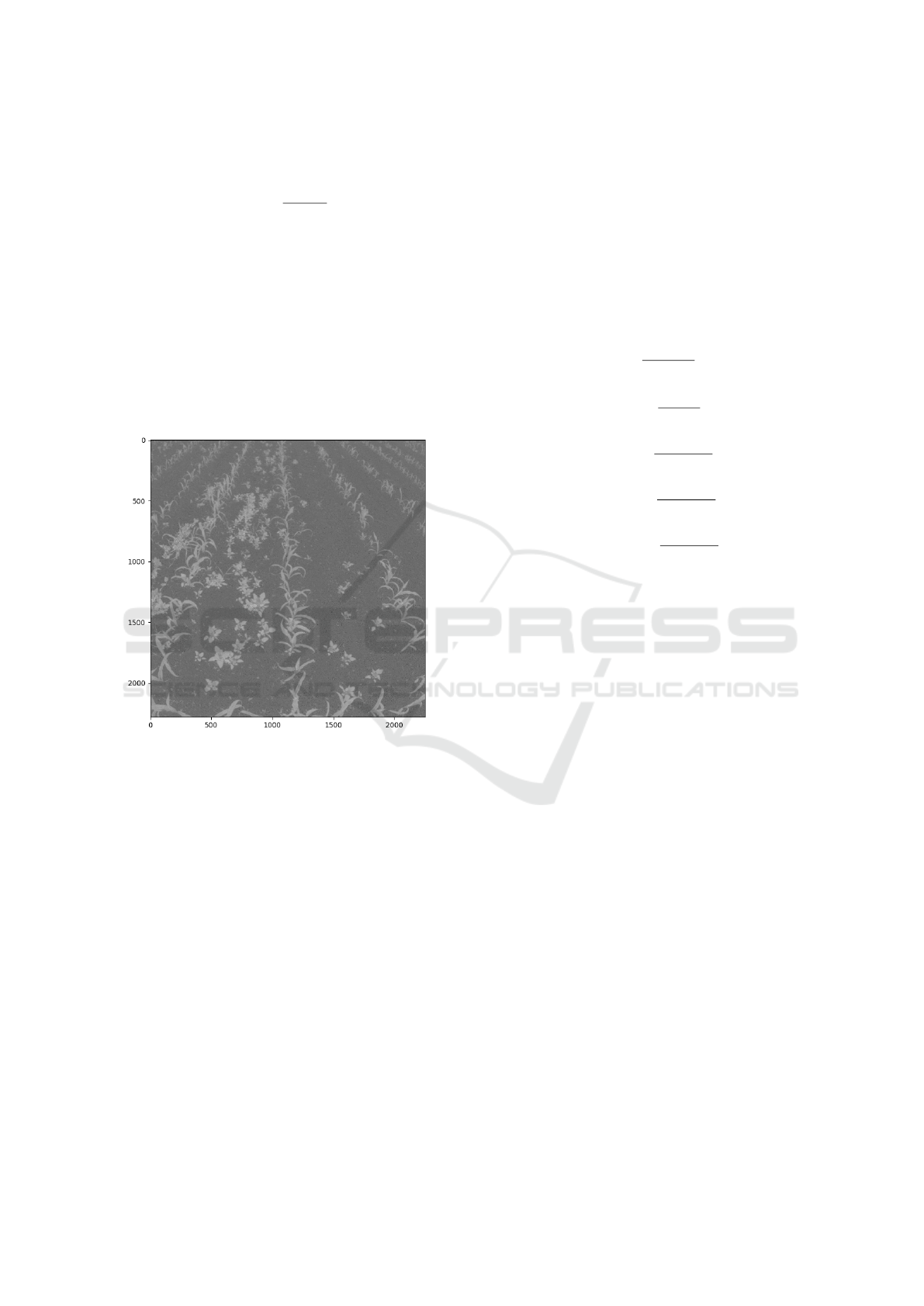
to reﬂect, respectively, red and green shades. Figure 1

shows an example of the MGRVI index obtained for

an image.

Figure 1: Example of the MGRVI index obtained for an

image.

3.2 Dataset

To evaluate the proposed method we considered four

datasets presented in (Riehle et al., 2020). Each

dataset contains 50 images and it was obtained us-

ing a different camera, resulting in a total of 200 im-

ages. The cameras used for the ﬁrst two sets were

“GoPro HERO6 BLACK” and “Parrot SEQUOIA +”

which originated the datasets, respectively, GP and

SE. These images were obtained by an autonomous

caterpillar robot “Phoenix”. The other data set called

K2 was obtained by the robot “TALOS” using a “Mi-

crosoft Kinect v2” camera and the fourth dataset was

made available by the University of Bonn using a “JAI

AD-130GE” camera. For all camera datasets images

have 2280 × 2256 pixels size in RGB format. The

datasets contain images of different plants (maize and

sugar beet) at various growth stages and vegetation

coverages.

3.3 Evaluation

We used ﬁve metrics to assess the performance of

the proposed segmentation approach: Dice coefﬁcient

(Equation 10), Jaccard index (Equation 11), Precision

(Equation 12), Sensitivity (Equation 13) and Speci-

ﬁcity (Equation 14). In these equation, A and B are,

respectively, the proposed and the expert’s segmenta-

tion images, T P is the number of true positives, FN

is the false negative and T N is the true negative.

Dice =

2|A ∩ B|

|A| + |B|

(10)

Jaccard =

|A ∩ B|

|A ∪ B|

(11)

Precision =

T P

T P + FN

(12)

Sensitivity =

T P

T P + FN

(13)

Speci f icity =

T N

T N + FP

(14)

4 EXPERIMENTS

In our experiments, we aimed to segment images in

each dataset in order to extract the regions contain-

ing plants from the background image. To accom-

plish that we computed all selected vegetation indices

for each image in the datasets. In the sequence, we

used the K-means method to group the pixels into

two classes (K = 2), i.e., Plant and Background. We

initialized the centroids with the highest and lowest

value present in the image for each index. This was

performed to avoid any randomness and to guarantee

the reproducibility of the algorithm. By associating

the clusters obtained from K-means with the original

pixel position, we obtain a binary image representing

the two clusters, i.e., a segmented image represent-

ing regions of plant and background. Additionally,

we used an opening morphological operation, with a

15 × 15 structuring element in square format, to re-

move small noises in the segmented image.

The selected 15 × 15 kernel size of the structur-

ing element was deﬁned manually and gradually. We

started with a 5 × 5 kernel size and we increased its

size as it kept reducing the presence of small noises

and improved the result. The decision to use a square

kernel was not based on any particular need, but due

to the fact this kernel is commonly used in morpho-

logical opening and closing operations.

VISAPP 2021 - 16th International Conference on Computer Vision Theory and Applications

508

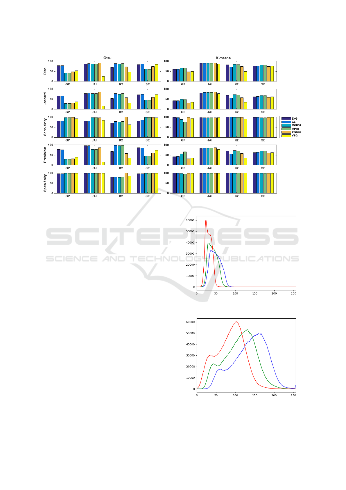
Figure 2: Comparison results for Otsu and K-means method for each vegetation index in all datasets.

Alternatively, we also evaluated the performance

of a simple automatic threshold approach to segment

the vegetation index images. In this case, we replaced

the K-means method in the approach previously de-

scribed by the Otsu method.

5 RESULTS

In this section, the results obtained by the experiments

conducted on this work were presented. Each vegeta-

tion index was applied to each dataset as explained

in Section 3. Figure 2 shows the results obtained in

each metric by each vegetation index in all datasets,

for both K-means and the Otsu method.

In general, the best results are obtained in the JAI

dataset. Images in this dataset present small varia-

tion in luminosity and brightness, increasing the ef-

fectiveness of segmentation, which is corroborated

by Dice coefﬁcients ranging from between 86.82% to

91.31%. We also notice that, for this dataset, the K-

means approach is slightly superior in comparison to

Otsu. Moreover, this dataset presents a small varia-

tion in green shades present in the plants and the soil

color pattern is very homogeneous (Figure 3). On the

other hand, the GP dataset presented, in general, the

worst results. This is explained due to the large varia-

tion of luminosity present in the images, as shown in

Figure 4. A superﬁcial analysis of the images in this

dataset shows there exists a variation in luminosity

caused by the local climate, as also an increase in the

Figure 3: Example of histogram of an image from JAI

dataset.

Figure 4: Example of histogram of an image from GP

dataset.

Segmentation of Agricultural Images using Vegetation Indices

509

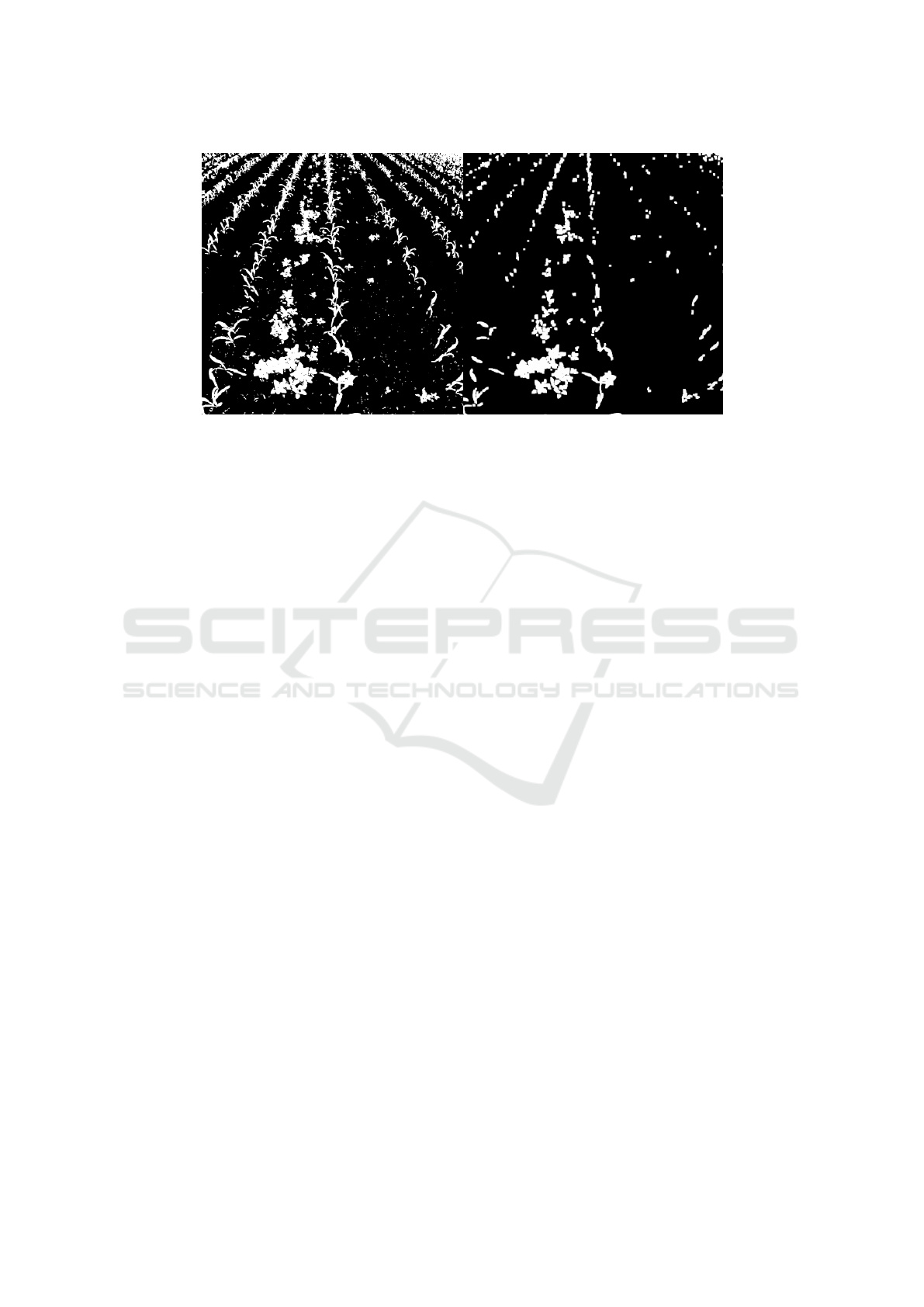
Figure 5: Noise reduction using morphological opening over the result of the K-means approach. Left: Binary image obtained

from segmentation. Right: Image after morphological opening.

image exposure due to differences in the reﬂection of

the sunlight by the soil. Even for images where there

was small light variation, as in the SE dataset, the dif-

ference in the reﬂection of light on the ground still

inﬂuences the results.

When comparing Otsu and K-means, we notice

that K-means tend to obtain higher results. For

the same dataset, Otsu presents higher oscillation in

their results depending on the vegetation index used.

Meanwhile, K-means, on average, presents similar re-

sults for different vegetation indices. This indicates

that the process of clustering can detect more efﬁ-

ciently different regions of interest (soil and plant)

than thresholding. This is partially explained by the

fact that K-means uses a distance metric to compute

the clusters and iteratively moves the centroid for the

positions that best separate the different classes of ob-

jects.

We must also emphasize the importance of mor-

phological opening, as shown in Figure 5. As one

can notice, this operation diminishes the level of noise

(e.g., loose pixels and other small objects) resulting

from the segmentation process.

Among all compared indices, MGRVI presented

the best results for the Dice coefﬁcient, ranging from

65.0% to 90.0%. This is a normalization of GRVI

whose vegetation and soil reﬂectance pattern is rela-

tively easy to interpret, where the vegetation reﬂects

the green band more than the red, while the soil re-

ﬂects the red band more than the green (Motohka

et al., 2010). Figure 6 shows the best segmentation

obtained using K-means for each dataset.

6 CONCLUSIONS

In this paper, we presented a study of different veg-

etation indices to segment plants/soil in images. We

evaluated two approaches to segment the images from

four different datasets: K-means and Otsu. Results

demonstrated the superiority of the K-means method

to segment these images when applied in combina-

tion with the MGRVI index. The evaluation carried

out by this work gives us an overview of the behav-

ior of each vegetation index for different types of

images (acquired at different conditions and equip-

ment) and their limitations, making it clear that a sin-

gle index may not be satisfactory to segment plants

from the background. In future work, we intend

to combine different vegetation indices to obtain a

more robust result for different datasets, to evaluate

whether the use of other color model (e.g., HSV)

combined with vegetation indices can improve the re-

sult obtained, and evaluate different automatic thresh-

old methods. We also intend to study the application

of vegetation indices that use multispectral images for

the plant/background segmentation process.

ACKNOWLEDGEMENTS

Andr

e R. Backes gratefully acknowledges the ﬁ-

nancial support of CNPq (Grant #301715/2018-1).

This study was ﬁnanced in part by the Coordenac¸

de Aperfeic¸oamento de Pessoal de N

ıvel Superior -

Brazil (CAPES) - Finance Code 001.

VISAPP 2021 - 16th International Conference on Computer Vision Theory and Applications

510

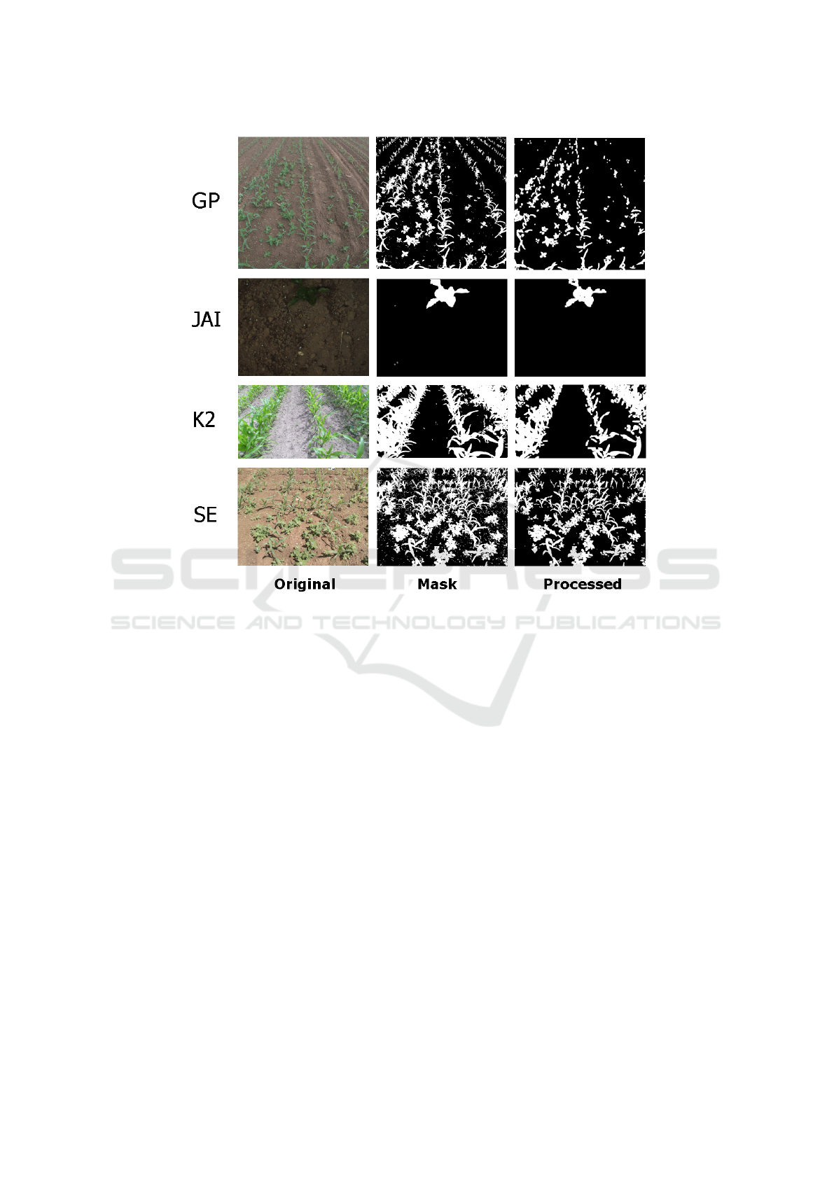
Figure 6: Best results obtained for each dataset. For datasets GP and K2, best results is obtained using MGRVI index. For

JAI dataset, best result is obtained using RGBVI, while MPRI index performs best in SE dataset.

REFERENCES

Abbasi, A. and Fahlgren, N. (2016). Na

ıve bayes pixel-level

plant segmentation. In 2016 IEEE Western New York

Image and Signal Processing Workshop (WNYISPW),

pages 1–4.

Bargoti, S. and Underwood, J. P. (2016). Image segmen-

tation for fruit detection and yield estimation in apple

orchards. CoRR, abs/1610.08120.

Bendig, J., Yu, K., Aasen, H., Bolten, A., Bennertz, S.,

Broscheit, J., Gnyp, M. L., and Bareth, G. (2015).

Combining uav-based plant height from crop surface

models, visible, and near infrared vegetation indices

for biomass monitoring in barley. International Jour-

nal of Applied Earth Observation and Geoinforma-

tion, 39:79 – 87.

Hague, T., Tillett, N., and Wheeler, H. (2006). Automated

crop and weed monitoring in widely spaced cereals.

Precision Agriculture, 7:21–32.

Louhaichi, M., Borman, M., and Johnson, D. (2001). Spa-

tially located platform and aerial photography for doc-

umentation of grazing impacts on wheat. Geocarto

International, 16.

Motohka, T., Nasahara, K., Hiroyuki, O., and Satoshi, T.

(2010). Applicability of green-red vegetation index

for remote sensing of vegetation phenology. Remote

Sensing, 2.

Otsu, N. (1979). A threshold selection method from gray-

level histograms. IEEE Transactions on Systems,

Man, and Cybernetics, 9(1):62–66.

Riehle, D., Reiser, D., and Griepentrog, H. W. (2020).

Robust index-based semantic plant/background seg-

mentation for rgb- images. Comput. Electron. Agric,

169:105201.

Woebbecke, D., Meyer, G., Bargen, K., and Mortensen, D.

(1995). Color indices for weed identiﬁcation under

various soil, residue, and lighting conditions. Trans-

actions of the ASAE, 38:259–269.

Yang, S., Wang, L., Shi, C., and Lu, Y. (2018). Evalu-

ating the relationship between the photochemical re-

ﬂectance index and light use efﬁciency in a mangrove

forest with spartina alterniﬂora invasion. International

Journal of Applied Earth Observation and Geoinfor-

mation, 73:778 – 785.

Zhuang, S., Wang, P., and Jiang, B. (2018). Segmentation

of green vegetation in the ﬁeld using deep neural net-

works*. In 2018 13th World Congress on Intelligent

Control and Automation (WCICA), pages 509–514.

Segmentation of Agricultural Images using Vegetation Indices

511