
Graph Convolution Networks for Cell Segmentation
Sachin Bahade, Michael Edwards and Xianghua Xie
Department of Computer Science, Swansea University, U.K.
Keywords:
Graph Convolution Network, Signal Processing, Cell Segmentation, Medical Imaging.
Abstract:
Graph signal processing is an emerging field in deep learning, aiming to solve various non-Euclidean domain
problems. Pathologist have difficulty detecting diseases at an early stage due to the limitations of clinical meth-
ods and image analysis. For more accurate diagnosis of disease and early detection, automated segmentation
can play a vital role. However, efficiency and accuracy of the system depends on how the model learned. We
have found that traditional machine-learning methods, such as clustering and thresholding, are unsuited for
precise cell segmentation. Furthermore, the recent development of deep-learning techniques has demonstrated
promising results, especially for medical images. In this paper, we proposed two graph-based convolution
methods for cell segmentation to improve analysis of immunostained slides. Our proposed methods use ad-
vanced deep-learning, spectral-, and spatial-based graph signal processing approaches to learn features. We
have compared our results with state-of-the-art fully convolutional networks(FCN) method and found a sig-
nificant of improvement of 2.2% in the spectral-based approach and 3.94% in the spatial-based approach in
pixel based accuracy.
1 INTRODUCTION
Humans are surrounded with data and it is present
everywhere. Such data have been processed. The
processing of data itself could be improved in order
to enhance the way social networks process data, or
to benefit the medical and financial sector, for exam-
ple. There are various techniques evolved in terms of
processing these data. In deep-learning, the convolu-
tional neural network has shown remarkable success
in various computer-vision problems such as segmen-
taion and classification (Badrinarayanan et al., 2017;
Krizhevsky et al., 2012). The reason behind these ac-
complishments is that data lies in the Euclidean do-
main, have locality and order information which fa-
cilitates the convolution operation learning represen-
tative features. These Euclidean data have the limi-
tation of generality when processed by conventional
convolutional neural networks, for example convo-
lution operation on a social-network graph. Data
which do not belong to the Euclidean space is known
as ’non-Euclidean’ or ’irregular’ domain data. One
of the solutions is that such non-Euclidean data can
be represented on the graph. The study of graph-
signal processing and spectral-graph theory works
with irregular-domain data and these studies have
helped to design tools for various operations like con-
volution and filtering on graph (Bronstein et al., 2017;
Sandryhaila and Moura, 2013). (Kipf and Welling,
2016) used graph-signal processing tools to formulate
convolution on graph as a multiplication of the sig-
nal with a filter in the Fourier domain (Shuman et al.,
2013). Another approach of graph-signal processing
is the spatial based graph convolution neural network,
where neighbouring information is gathered around a
centre node to process operations.
An image is usually considered as an array of pixel
values arranged in a 2D grid form. The data arranged
in this fashion can also be considered as a signal ly-
ing on a 2D grid graph, where pixel values lie on each
node as features. The connectivity of pixel neigh-
bourhoods is represented by an adjacency matrix de-
scribing the connectivity between pixels. This pixel
connectivity of an image in a 2d grid graph helps to
solve segmentation problems. The most used meth-
ods for these tasks are fully convolutional network
(FCN) (Long et al., 2015) and U-Net (Ronneberger
et al., 2015). These architectures are primarily based
upon convolutional neural network(CNN), where a
FCN requires more training data and the U-Net is de-
signed for biomedical images with few samples and
enough time with no dense layer. Our contribution
in this paper is to apply a graph convolution opera-
tor on the non-Euclidean data and propose a method
for segmentation task on biomedical cell image data.
We have experimented these data with different tra-
620
Bahade, S., Edwards, M. and Xie, X.
Graph Convolution Networks for Cell Segmentation.
DOI: 10.5220/0010324306200627
In Proceedings of the 10th International Conference on Pattern Recognition Applications and Methods (ICPRAM 2021), pages 620-627
ISBN: 978-989-758-486-2
Copyright
c
2021 by SCITEPRESS – Science and Technology Publications, Lda. All rights reserved

ditional methods like clustering, threshold and deep
learning methods such as FCN, spectral and spatial-
based graph convolution. In observation, we have
found that graph convolution networks improve seg-
mentation results. This paper is divided into the fol-
lowing sections. Section II provides a review of cell
segmentation and related deep-learning methods. In
Section III, our proposed graph-CNN architecture and
method is discussed. In section IV, we show the
implementation of the threshold-based Otsu method,
the k-means clustering method, and the deep-learning
and graph-based methods, to solve the same prob-
lem. In the results section, our method is qualitatively
and quantitatively compared with the state-of-the-art
FCN. Section VI concludes the paper.
2 RELATED WORK
In the medical field, lymphoma cancer cells found
important elements that is a cluster of differentia-
tion 4 (CD4) and cluster of differentiation 8 (CD8)
where CD8 helps to kill infected virus cells and CD4
works as a signal activator. In a clinical setting,
the CD4/CD8 count ratio is used to judge the condi-
tion of the immune system. Automated segmentation
of such immunostaining images helps to carry out a
more accurate diagnosis of disease or even early de-
tection (Ronneberger et al., 2015). A review of var-
ious automated methods for cell detection and seg-
mentation is provided by (Thomas and John, 2017).
There are several approaches used for segmentation
including traditional and deep learning. Mainly we
are focusing on graph based approach convolution op-
eration to understand node based features.
2.1 Traditional Methods for
Segmentation
One approach for image segmentation is developed
using principal component analysis (PCA) and k-
means (Katkar et al., 2016). In order to identify tuber-
culosis bacteria, (Rulaningtyas et al., 2015), devel-
oped a new algorithm to help clinicians. They identify
the problem of local minima in k-means and solved
it by windowing technique. The whole image is di-
vided into small patches and segment each patch is
segmented using k-means clustering.
There is a feature classification limitation of a
region-, edge-, and pixel-based segmentation with
color images. By transferring the RGB image into
CIELAB (L*a*b) color space, (Yadav et al., 2016)
analyze the features of each pixel of an image, classi-
fying the colors using k-means and adopting support
vector machine (SVM) classifiers to detect tumours
by comparing the clustered image with labelled data.
The two-colour components, a and b, from L*a*b
colour space can also be used as a feature for k-means
clustering in the segmentation of white blood cells
from microscopic images (Salem, 2014). Another
approach to obtain segmentation of white blood cells
for acute leukaemia images is to use a linear-contrast
segmentation technique using hue, saturation and in-
tensity (HSI) colour space (Abdul Nasir et al., 2011).
Recently there has been a growth in the use of
deep learning techniques for medical-image analysis,
especially segmentation tasks for the early detection
of disease. (Wang et al., 2016) used deep learning
techniques with the threshold-based Otsu method to
identify tissue: dividing image into patches and ap-
plying supervised classification to detect a tumour.
Some of the promising works on deep learning for im-
age segmentation tasks gain most researchers’ atten-
tions (Ronneberger et al., 2015; Badrinarayanan et al.,
2017; Arora and Patil, 2017; Abdul Nasir et al., 2011;
Long et al., 2015).
2.2 Deep Learning based Segmentation
One of the state-of-the-art deep learning methods
used in this study is FCN-based segmentation (Long
et al., 2015). It is an encoder-decoder architecture
made by fine-tuning a portion of the VGG-16 network
and it does not have a dense layer. It is replaced with
1 ×1 convolution to adapt the classifier for dense pre-
diction, to classify each pixel within an image and as-
sign a label to them. To get the output size equal to
the original size, upsampling is used to expand the
features. There might be information loss through the
convolution process, so skip connection helps to re-
cover lost information (Long et al., 2015). (Arora
and Patil, 2017) adapt a model from (Laina et al.,
2016) and used transfer learning to solve the problem
of depth prediction of a scene from a single monoc-
ular image and pixel-wise semantic labelling. The
popular SegNet architecture (Badrinarayanan et al.,
2017) eliminates the need for learning to upsample
compared to FCN. U-net architecture is build based
on FCN architecture (Ronneberger et al., 2015). The
only difference is that the pooling operation of up-
sample part is replaced by up-convolution which in-
creases the resolution and concatenates skip connec-
tion instead of adding, helping to improve segmenta-
tion.
Graph Convolution Networks for Cell Segmentation
621
2.3 Graph-based Convolutional Neural
Networks
The popularity of graph-based convolutional neural
networks has been rapidly growing in recent years due
to the generic nature of irregular data. Graph con-
volution updates the node based on the neighbouring
node information and processed for the convolution
operation. Graph convolution networks is categorised
into two forms: spectral-, and spatial-based. Spectral-
based convolution uses filters from the perspective of
graph-signal processing while spatial-based convolu-
tion defines graph convolutions by information prop-
agation.
The Graph is a set of vertices and edges where
nodes are connected. Graph convolution is the con-
volution operation in the frequency domain. The ma-
trix representation of the graph is convolved with the
features matrix. The result multiply with the weights
W
i
on each nodes in the i
th
layer and passed through
the hidden layer non-linear function. In conventional
CNN, the pooling layer is used to reduce the resolu-
tion of input feature map but in the case of a graph,
there is no reduction of size due to the multiplication
of the filter with spectral signal (Edwards and Xie,
2016). To pool local feature output from the convo-
lution layer, it is required to perform graph coarsen-
ing which reduces the number of vertices, and handle
the edges between these vertices based on the similar
properties. In graph convolution, there is no reduction
of vertices, only changes in the output filter channel.
But for the precise classification, pooling generalizes
features in the spatial domain. Agglomerative pool-
ing is a bottom-up approach to reduce vertices and
project the features on a new graph. There are various
methods to do graph coarsening such as graclus etc.
One of the common methods for selecting vertices is
to select a subset of the set of vertices or generate
new nodes. Algebraic Multigrid (AMG) is a graph
coarsening method which project a signal to a coarser
graph by greedy selection of vertices. This method is
used as a pooling operation on graph (Edwards and
Xie, 2016).
Spatial-based graph convolution follows the simi-
lar approach of convolutional operation of a conven-
tional CNN on an image. Their operation is based
on a node’s spatial relations. Images are represented
as a special form of 2D graph with each pixel repre-
senting a node and is directly connected to its nearby
pixels. Similar to conventional convolution operation,
spatial graph convolution perform convolution opera-
tion by considering its neighbours representations of
node and central node.
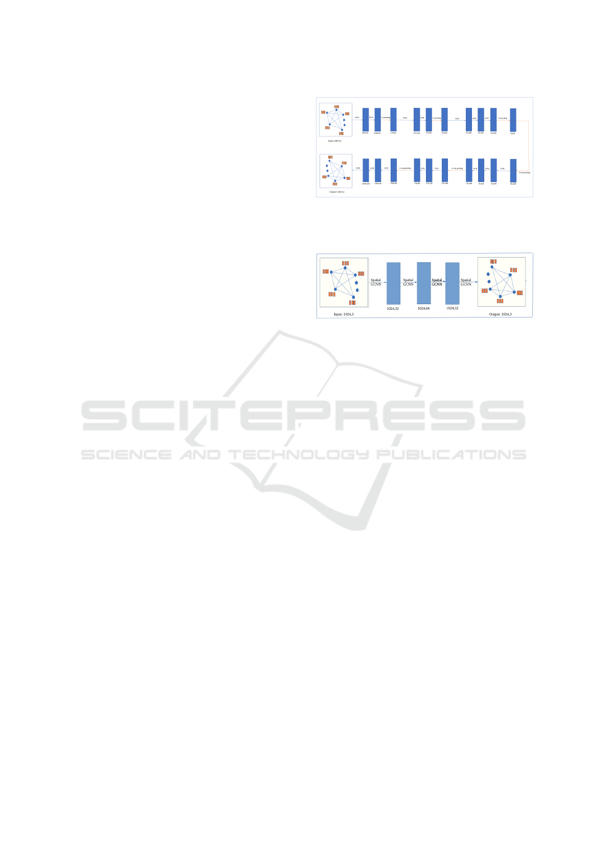
Figure 1: GCNN architecture: blue color box represents
output result of the graph, processed by operations GCN/G-
pooling. It also mentioned the size of the graph: number of
nodes and output channels.
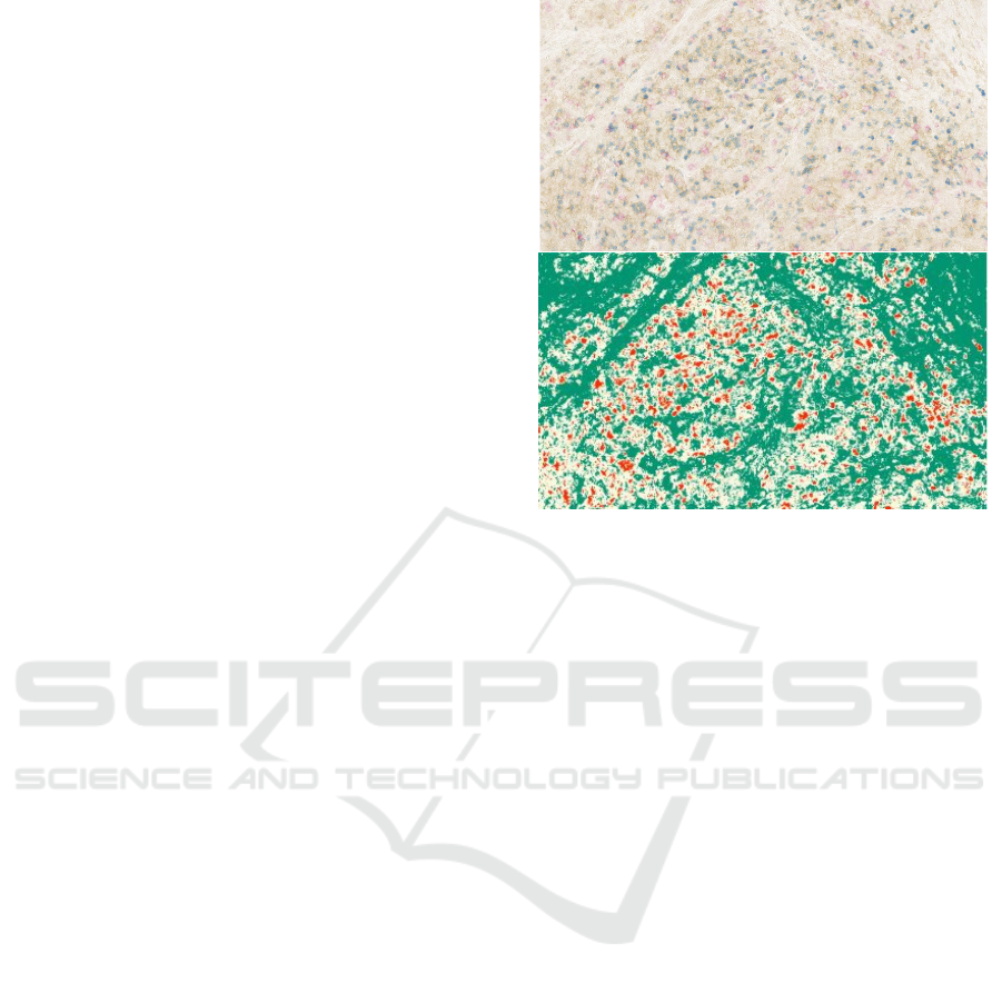
Figure 2: Spatial GCNN architecture: blue color box rep-
resents output result of the graph, processed by operations
spatial GCNN. It also mentioned the size of the graph: num-
ber of nodes and output channels.
3 METHODS
3.1 Proposed Network Architecture
Motivated by the convolution neural network U-net
architecture, we propose a similar architecture us-
ing spectral based graph convolution and graph pool-
ing. The network architecture is illustrated in Fig-
ure 1. The encoder part consists of its three blocks,
each consisting of three graph convolutions and graph
pooling layers. For graph-pooling operation, we uti-
lize AMG coarsening to obtain the restriction and
projection matrices. The decoder part starts with
the graph up-pooling operation in sequence with the
last pooling operation of an encoder. It consists of
three layers of graph convolution, each initiated with a
graph up-pooling operation. In the case of up-pooling
operation, we used the projection matrix of previous
coarsened graph to reconstruct original size graph di-
mension.
In the spatial approach based graph convolution
architecture, we have used mixture model CNN
(MoNet) framework for the graph convolution oper-
ation where each convolution operation is followed
by activation. Here we have avoided the pooling
operation as the spatial approach used aggregative
methods of neighbour node used to learn efficiently
large graphs.
ICPRAM 2021 - 10th International Conference on Pattern Recognition Applications and Methods
622

3.2 Proposed Method of Utilizing
Spectral based Graph-CNN
To perform convolution on the graph, spectral theory
is used to define the analogue to convolution and for
the downsampling and upsampling operation, graph
coarsening as a pooling layer is defined. While per-
forming the graph pooling, we partition the graph
into coarsened graph and use projection and restric-
tion for graph pooling and graph up pooling opera-
tion (Liu et al., 2014) (Masci et al., 2015). Training is
fed forward through the network to obtain output and
loss propagates backward to update the weights. The
graph holds spatial information about the connectivity
of nodes and allows graph processing tools, convolu-
tion and pooling, to operate on signals (Shuman et al.,
2013).
To perform the graph convolution, an image is
considered as a 2D grid graph, having a set of nodes
(V ), set of weighted edges (E) and adjacency matrix
(A). The graph possesses the property that each node
is connected with its neighbouring nodes which form
the basis of locality for the convolution operation.
The graph structure of the image represents an
irregular data and graph Laplacian is the core op-
erator for graph convolution layer. One form of
the Laplacian operation is represented as L = D − A
where D is the degree matrix and A is the adjacency
matrix. Normalized Laplacian matrix is L = I
n
−
D
−1/2
AD
−1/2
where I
n
is the identity matrix which
considers self node features. The Laplacian matrix
is decomposed into orthonormal vector U = u
i=1...N
where u
i
is eigenvector associating with eigenvalues
λ
i=1...N
. Apply graph Laplacian and then eigende-
composition of graph Laplacian matrix which gives
the Fourier modes and graph frequencies (Defferrard
et al., 2016). In graph signal processing, a graph sig-
nal
0
s
0
is a feature vector that lies on the node of the
graph. Applying the graph Fourier transform (F
G
) us-
ing matrix U on signal s gives,
F
G
(s) = ˆs = U
T
s (1)
Then the inverse graph Fourier transform is applied
which gives original signal s (Defferrard et al., 2016),
F
−1
( ˆs) = U ˆs = UU
T
s = s, (2)
Now the convolution of signal s with a filter g in
Fourier domain is defined as,
s ∗
G
g = F
−1
G
(F
G
s F
G
g), (3)
and can be represented in,
s ∗
G
g = ˆg(L)s, (4)
For the graph pooling operation, we are using the
AMG method to coarsen a graph and projecting sig-
nals on a new coarsened graph via a greedy selection
of vertices (Chevalier and Safro, 2009). The two-level
coarsening is shown in the Figure 5. Every AMG
coarsened graph provides the restriction matrix R and
the projection matrix P for the interpolation of the in-
put signal s. Downsampling operation is performed
by multiplication of signal and restriction matrix
s
j
= s
i
∗ R
i
and reverse pooling by multiplication with projection
matrix,
s
i
= s
j
∗ P
j
Where s
j
is the output of the downsampling operation
and s
i
is the output of up-sampling. R
i
and P
j
are the
restriction and projection matrices, respectively.
3.3 Proposed Method of Utilizing
Spatial based Graph-CNN
Similar to the conventional CNN on the two dimen-
sional grid image, spatial based graph convolution de-
fines the spatial relation of the node and its neighbour-
ing nodes on the graph. Each node is represented as
a vertex of the graph, and the value is the signal on
that vertex. In the spatial graph convolution network,
centre nodes are updated by averaging the neighbours
nodes analogous to the conventional CNN.
In our case, we are using a spatial based mixture
model CNN for graph (MoNet) where the pixel neigh-
borhood relationship can be represented by a pseudo-
coordinate. In this approach, x represents a vertex on
a graph, and yεN(x) are the vertices in the neighbour-
hood of x. Assign a d dimensional vector of pseudo-
coordinate u(x, y). The pseudo-coordinate calculates
the degree of nodes by the equation
u(x,y) = (1/
p
deg(x),1/
p
deg(y))
T
(5)
In this coordinate space, parametric learnable gaus-
sian kernel function is defined as below:
W
j
(u) = exp(−1/2(u − u
j
)
T
(Σ
j
)
−
1(u − u
j
)) (6)
where Σ
j
and u
j
are learnable d × d and d × 1 covari-
ance matrix and mean vector of Gaussian kernel.
With the help of these kernel function, a patch op-
erator is used to perform the function of convolution
operation. This operator applies the Gaussian ker-
nel on each node pseudo-coordinate with all neigh-
bourhood and summoned up the results (Monti et al.,
2017).
D
j
(x) f =
∑
yεN(x)
w
j
(u(x,y)) f (y), j = 1,...J, (7)
The patch operator can be defined by the above
equation, Where J represents the dimensionality of
Graph Convolution Networks for Cell Segmentation
623
extracted patch. The generalised graph convolution
operation is written as
( f ∗ g)(x) =
J
∑
j=1
g
j
D
j
(x) f , (8)
where g
j
is the learnable weight matrix.
4 EXPERIMENTATION
4.1 Generation of Hodgkin Lymphoma
(Ground Truth) Segmentation
The microscopic immunostaining images of Hodgkin
lymphoma show some patterns of stain based on the
colour of those stains. The slide is stained with
two immunostaining patterns CD4 and CD8. How-
ever, the data need to be cleaned to overcome a large
amount of additional noisy information. To create a
ground truth label for segmentation, manual labelling
of each cell is created by selecting the contour points
for each cell class and all the pixels are filled inside
the contour with the unique class ID. In this way, the
ground truth label is the same size image where every
pixel is assigned a class label. It can also be described
as dense labelling.
Further, the labelled data we have created is used
for supervised machine learning, to learn meaningful
features from the data and used in deep learning ex-
perimentation.
4.2 Segmentation using Clustering
Method
Clustering plays an important role in segmentation.
There are many methods that have been proposed for
segmentation. Among them, k-means becomes very
popular. Due to good results of the k-means clustering
method (Katkar and Baraskar, 2015), we have chosen
this method for our data and the result is shown in Fig-
ure 3. k, the number of clusters chosen is three. K-
means identifies the nearest pixels assign to random
centroid and shifts centroid to a new position based
on the average of pixels in the cluster. The output im-
age shows the segmentation of CD4, CD8 and back-
ground.
4.3 Segmentation using Deep Learning
We used fully convolutions neural network as one of
the state-of-the-art methods for segmentation. We
prepared the data and created patches of size 224 ×
Figure 3: K-Means clustering of Hodgkin lymphoma im-
munostaining image. Top: Original image, Bottom: Seg-
mentation via k-means. red colors represent a CD4, yellow
shows CD8 and rest are background FOXP3 protein.
224 from 768 ×1366 size image. With the deep learn-
ing supervised approach, we need data images as well
as respective class label masks for each patch.
In this architecture, the encoder contains several
layers. Each layer is a combination of convolution
followed by pooling operation. At each convolu-
tion, 3 × 3 kernel convolve with the input image and
produces output feature maps. The decoder is used
to reconstruct the original image by upsampling and
skip connection. In the experimentation, initially
224 × 224 size patches fed into the network. The in-
tersection oven union (IOU) accuracy was observed
with varying accuracy when it was tested on the un-
seen image. The resulting output obtained from this
fine-tuning is shown in Figure 4. Pixel based accu-
racy was found to be accuracy 0.8709 %, trained with
Adam optimizer and learning rate of 0.001. We have
used a total of 414 patch samples for training and val-
idation.
4.4 Segmentation using Spectral
Graph-CNN
Due to the resource limitation required for the spec-
tral based graph convolution, the original image was
divided into patches of size 32 × 32 × 3. To process
this patch using the graph, first we need to construct
the graph which holds the signal that is 32 × 32 × 3
size. Let N be the number of nodes holding the 3
RGB pixel values at each node say d. The mathe-
ICPRAM 2021 - 10th International Conference on Pattern Recognition Applications and Methods
624
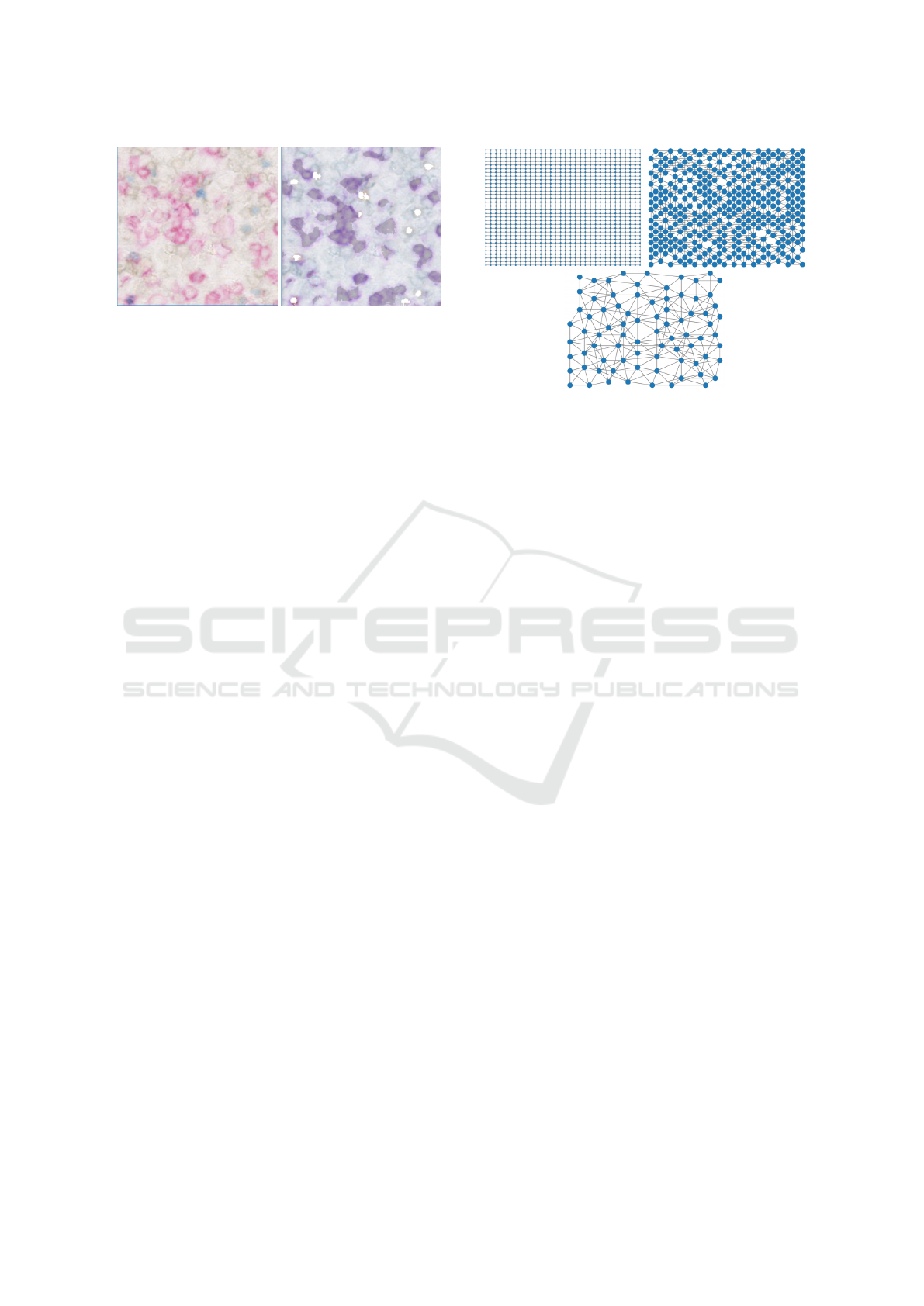
Figure 4: Left: Original Image, Right: FCN Fine-Tuning
method.
matical form of graph convolution operation is men-
tioned in section 3.2. However, simplified expression
of graph convolution operation explained here. This
expression is nicely derived from spectral base graph
convolution (Kipf and Welling, 2016). X is a feature
matrix of dimension N ×F
0
. N is the number of nodes
and F
0
is the number of features on each node. The
2D grid graph is created to hold this signal, with the
dimension N ×N. This N ×N binary matrix stores the
connectivity of the node, and is called as adjacency
matrix represented by A. Like conventional CNN, the
hidden layer in graph-CNN is represented by
H
i
= f (H
i−1
,A) (9)
as H
i
is i
th
hidden layer. For optimization and
training, weight is assign to edges between connect-
ing nodes as weight matrix W
i
and also consider the
self node features that are added into the adjacency
matrix. So, the new adjacency matrix is,
ˆ
A = A + I
where I is an identity matrix. Graph convolution is
modified as, first compute the node feature represen-
tation of each node by aggregating feature represen-
tation of its neighbours node and then transform it by
multiplying by the weight matrix. To avoid the gradi-
ent exploding, normalize the feature representation by
adding degree matrix D
−1
. Whole graph convolution
is represented as,
f (H
i
,A) = σ(D
0.5
AD
0.5
H
i
W
i
) (10)
where σ is a nonlinear activation function. The
Laplacian matrix is decomposed into orthonormal
vector U . This eigendecomposition of graph Lapla-
cian gives the Fourier mode and graph frequencies.
So, the generalized equation of graph convolution is,
f (H
i
,A) = σ(U ∗ s) (11)
where, s is a signal on a graph.
4.5 Segmentation using Spatial
Graph-CNN
In the experimentation of spatial graph CNN we are
using a MoNet operator as described in the method
Figure 5: Graph representation: Top left: Original graph
of the 2D grid, Top right: first coarsening level with AMG
pooling, Bottom: second coarsening level with AMG.
section. We have set the neighbourhood of each ver-
tex is 4 and based on the Euclidean distance their
respective four adjacent nodes has been collected in
sorted order and build an adjacency matrix of k near-
est neighbour graph. To perform a Gaussian ker-
nel operation, coordinate distance between source and
target node is used as a pseudo-coordinates. In the op-
eration, apply Gaussian kernel w
j
(u(x,y)) over each
pseudo coordinate on the nodes and their neighbours
yεN(x) the result is multiplied with the signal on
neighbour f (y) and summed all the neighbours re-
sults. We have used Gaussian kernel size 25 and
summed up the result of each Gaussian output patch.
All operations are defined as the patch operator. This
patch operator multiplied with the learnable weight
matrix to perform convolution operation.
( f ∗ g)(x) =
J
∑
j=1
g
j
D
j
(x) f , (12)
Here g is the weighted matrix and D
j
(x) is patch op-
erator.
The architecture used in the model contains 4
graph convolution blocks with output feature size
32, 64, 32 and 3, giving the segmented output same
as input dimension. Each layer is followed with
LeakyRelu activation function except the last layer.
In the architecture diagram 2, the blue box shows the
output graph with the number of nodes and feature
size and edges describes the convolution operation.
For the training, ten thousand random patches from
each image size 1366 × 768 graph signal, has col-
lected for 21 such images patches. The data is trained
with 5 fold cross validation with RMSProp optimizer
and learning rate of 1e-5. We have set the the training
epoch 10 with batch size one that helps to enhance the
functionality of patch operator and learn the feature
Graph Convolution Networks for Cell Segmentation
625
better as compare to spectral based graph convolution
as shown in confusion matrix Figure 6.
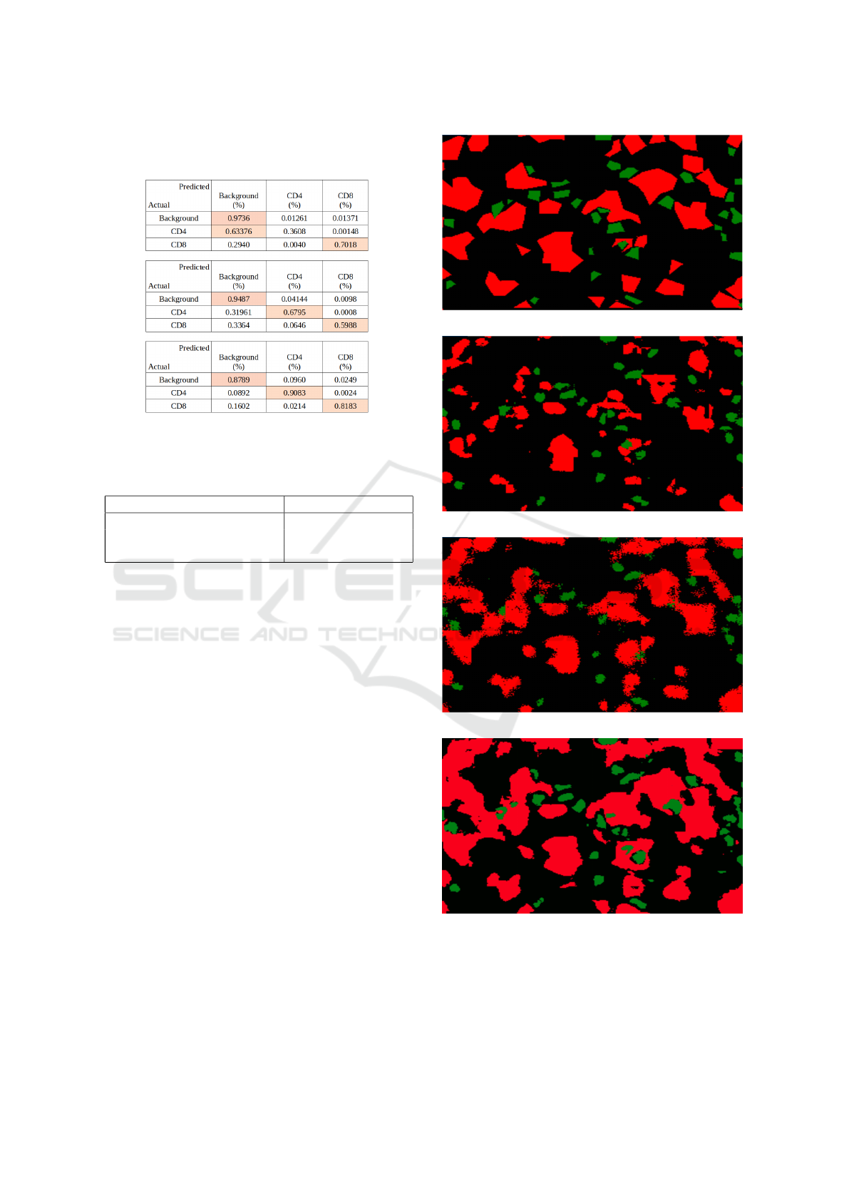
Figure 6: Confusion Matrices of segmentation methods.
Top: FCN, Middle: Spectral Graph-CNN, Bottom: Spatial
Graph-CNN.
Table 1: Quantitative comparison of results.
Method Pixel Accuracy (%)
FCN 87.09
(Ours)Spectral Graph-CNN) 89.29
(Ours)Spatial Graph-CNN) 91.03
5 RESULT
For training and testing we have used a total of 23
images of size 1366 × 768 cell segmentation dataset.
For FCN approach training and validation data sam-
ple is divided into ratio of 70:30 for the total 414
patch samples. We report the average accuracy of
87.09% computed over a total of 18 patch samples of
size 224 ×224. Regarding the graph-based approach:
due to limitation of resources we used samples of
size 32 × 32 and total number of sample for training
and validation is 30800 with 70:30 ratio. The pixel
accuracy is taken over 1008 unseen image samples
for both spectral- and spatial-based approach with an
improvement of 2.2% and 3.94% compared with the
FCN approach. Their class based comparative analy-
sis of quantitative measure can be shown in the confu-
sion matrix of Figure 6 where both spectral and spatial
based methods shows significant improvement.
The comparative quantitative and qualitative
result of the proposed method is shown in Table 1
and Figure 7. It is observed that the size feature of
the cell is better represented by graph-based approach
with an improved result.
(a) Ground Truth
(b) FCN result
(c) Spectral G-CNN result
(d) Spatial G-CNN result
Figure 7: Qualitative Comparison of Results. 7a: Ground
Truth of original image of different samples, 7b: Result ob-
tained by FCN method, 7c: Result obtained by G-CNN
method, 7d:Result obtained by Spatial G-CNN method.
Red color represent the CD4 stain cells and Green color cor-
responds to CD8.
ICPRAM 2021 - 10th International Conference on Pattern Recognition Applications and Methods
626

6 CONCLUSIONS
This study proposes a novel method of performing
segmentation on cell images using spectral and spa-
tial graph-CNN. It also allows patch-wise distribu-
tion of the original image for better feature learning.
Convolutions are performed in the spectral domain of
the graph Laplacian for learning of spatially localized
features. Spatial based graph convolution handles dif-
ferent graphs to learn locally, each node. Results are
provided on both conventional CNN and graph-based
CNN which shows graph-based CNN has the ability
to learn localized feature maps across multiple layers
of a network.
REFERENCES
Abdul Nasir, A. S., Mashor, M. Y., and Rosline, H.
(2011). Unsupervised colour segmentation of white
blood cell for acute leukaemia images. In IEEE In-
ternational Conference on Imaging Systems and Tech-
niques, pages 142–145.
Arora, Y. and Patil, I. (2017). Fully convolutional network
for depth estimation and semantic segmentation.
Badrinarayanan, V., Kendall, A., and Cipolla, R. (2017).
SegNet: A deep convolutional encoder-decoder archi-
tecture for image segmentation. IEEE Pattern Analy-
sis and Machine Intelligence, 39(12):2481–2495.
Bronstein, M. M., Bruna, J., LeCun, Y., Szlam, A., and Van-
dergheynst, P. (2017). Geometric deep learning: going
beyond euclidean data. IEEE Signal Processing Mag-
azine, 34(4):18–42.
Chevalier, C. and Safro, I. (2009). Comparison of coars-
ening schemes for multilevel graph partitioning. In
International Conference on Learning and Intelligent
Optimization, pages 191–205.
Defferrard, M., Bresson, X., and Vandergheynst, P. (2016).
Convolutional neural networks on graphs with fast lo-
calized spectral filtering. In Advances in neural infor-
mation processing systems, pages 3844–3852.
Edwards, M. and Xie, X. (2016). Graph based convolu-
tional neural network. In British Machine Vision Con-
ference.
Katkar, J., Baraskar, T., and Mankar, V. R. (2016). A novel
approach for medical image segmentation using PCA
and k-means clustering. In International Conference
on Applied and Theoretical Computing and Commu-
nication Technology, pages 430–435.
Katkar, J. A. and Baraskar, T. (2015). Medical image
segmentation using PCA and k-mean clustering algo-
rithm. In Post Graduate Conference for Information
Technology, pages 1–6.
Kipf, T. N. and Welling, M. (2016). Semi-supervised clas-
sification with graph convolutional networks. CoRR,
abs/1609.02907:1–14.
Krizhevsky, A., Sutskever, I., and Hinton, G. E. (2012). Im-
agenet classification with deep convolutional neural
networks. In Neural Information Processing Systems,
pages 1097–1105.
Laina, I., Rupprecht, C., Belagiannis, V., Tombari, F., and
Navab, N. (2016). Deeper depth prediction with fully
convolutional residual networks. 3D Vision, pages
239–248.
Liu, P., Wang, X., and Gu, Y. (2014). Graph signal coarsen-
ing: Dimensionality reduction in irregular domain. In
IEEE Global Conference on Signal and Information
Processing, pages 798–802.
Long, J., Shelhamer, E., and Darrell, T. (2015). Fully
convolutional networks for semantic segmentation.
In Computer Vision and Pattern Recognition, pages
3431–3440.
Masci, J., Boscaini, D., Bronstein, M. M., and Van-
dergheynst, P. (2015). ShapeNet: convolutional neu-
ral networks on non-euclidean manifolds. CoRR,
abs/1501.06297.
Monti, F., Boscaini, D., Masci, J., Rodola, E., Svoboda, J.,
and Bronstein, M. M. (2017). Geometric deep learn-
ing on graphs and manifolds using mixture model
cnns. In Computer Vision and Pattern Recognition,
pages 5115–5124.
Ronneberger, O., Fischer, P., and Brox, T. (2015). U-net:
convolutional networks for biomedical image segmen-
tation. Lecture Notes in Computer Science (including
subseries Lecture Notes in Artificial Intelligence and
Lecture Notes in Bioinformatics), 9351:234–241.
Rulaningtyas, R., Suksmono, A. B., Mengko, T., and
Saptawati, P. (2015). Multi patch approach in k-
means clustering method for color image segmenta-
tion in pulmonary tuberculosis identification. In Inter-
national Conference on Instrumentation, Communica-
tions, Information Technology, and Biomedical Engi-
neering, pages 75–78.
Salem, N. M. (2014). Segmentation of white blood cells
from microscopic images using k-means clustering. In
National Radio Science Conference, pages 371–376.
Sandryhaila, A. and Moura, J. M. (2013). Discrete signal
processing on graphs. IEEE Transactions on Signal
Processing, 61(7):1644–1656.
Shuman, D. I., Narang, S. K., Frossard, P., Ortega, A., and
Vandergheynst, P. (2013). The emerging field of signal
processing on graphs: Extending high-dimensional
data analysis to networks and other irregular domains.
IEEE Signal Processing Magazine, 30(3):83–98.
Thomas, R. M. and John, J. (2017). A review on cell detec-
tion and segmentation in microscopic images. In In-
ternational Conference on Circuits, Power and Com-
puting Technologies, pages 1–5.
Wang, D., Khosla, A., Gargeya, R., Irshad, H., and Beck,
A. H. (2016). Deep learning for identifying metastatic
breast cancer. CoRR, abs/1606.05718.
Yadav, H., Bansal, P., and Kumarsunkaria, R. (2016). Color
dependent k-means clustering for color image seg-
mentation of colored medical images. In Proceed-
ings on International Conference on Next Generation
Computing Technologies, pages 858–862.
Graph Convolution Networks for Cell Segmentation
627
