Dynamic and Scalable Deep Neural Network Verification Algorithm
Mohamed Ibn Khedher
1
, Hatem Ibn-Khedher
2
and Makhlouf Hadji
2
1
IRT - SystemX, 8 Avenue de la Vauve, 91120 Palaiseau, France
2
Universit
´
e de Paris, Lipade, F-75006 Paris, France
Keywords:
Feed-forward Neural Network, Neural Network Verification, Big-M Optimization, Robustness.
Abstract:
Deep neural networks have widely used for dealing with complex real-world problems. However, a major
concern in applying them to safety-critical systems is the great difficulty in providing formal guarantees about
their behavior. Verifying its behavior means study the evolution of its outputs depending on the variation of
its inputs. This verification is crucial in an uncertain environment where neural network inputs are noisy.
In this paper, we propose an efficient technique for verifying feed-forward neural networks properties. In
order to quantify the behavior of the proposed algorithm, we introduce different neural network scenarios to
highlight the robustness according to predefined metrics and constraints. The proposed technique is based
on the linearization of the non-convex Rectified Linear Unit (ReLU) activation function using the Big-M
optimization approach. Moreover, we contribute by an iterative process to find the largest input range verifying
(and then defining) the neural network proprieties of neural networks.
1 INTRODUCTION
Deep Neural networks have been widely used in many
applications(Jmila et al., 2019) , such as image classi-
fication (Khedher et al., 2018), telecommunications,
robot navigation and control of autonomous systems
(Bunel et al., 2018).
Currently, despite the huge effort in deep neural net-
works deployment in real time applications, the over-
all configuration requires an intelligent tuning process
across the input/output bounds that can secure and
verify the final constraints.
Taken the example of real-time autonomous sys-
tem, Deep Neural Networks (DNN) can be used for
several tasks :
• The perception of a vehicle: detection and recog-
nition of obstacles such as pedestrians, traffic
signs, road markings, etc.
• Driver status monitoring: eye direction, head an-
gle, heart and respiratory rates, etc.
• Decision-making depending on the environment
of a vehicle: lane change, speed and steering an-
gle calculation, etc.
It is worth mentioning here that in most application
fields, the predicted decision of neural networks (i.e.,
detecting the presence/absence of a pedestrian, chang-
ing or keeping the lane, etc.) has a serious impact on
the safety of the driver, the safety of passengers and
other users of the road. For instance, detecting the
absence of the pedestrian while he is actually present
can cause a serious accident.
Despite the power of Deep Neural Networks that
can process large inputs, analyse big data, and recom-
mend some tuning or decisions, the slight perturba-
tion in the input space can lead to a bad decision and
worst use cases (Bunel et al., 2018). These poor de-
cisions are generally caused by the disruption of the
environment, hence the need for a share of metrics al-
lowing the evaluation of the Neural Network to keep
security proprieties faced the uncertainty of the envi-
ronment.
The study of the security of a DNN consists in ver-
ifying the capacity of the Neural Network to take the
same decision for all similar data, despite the attacks
they can undergo. An attack is defined as any noise
that can disrupt the neural network. The checker (the
system verifying the security of the DNN) takes an
input, a data and an attack, and delivers an informa-
tion in the form of ”secure data faced the attack” or
”non-secure data faced the attack”. Therefore, a Neu-
ral Network Verification (NNV) approach is needed to
provide robustness metrics to neural networks.
The principle of Neural Network Verification is to
find out, from the input data, all possible data result-
ing from the attack (noisy data), and verify that the
1122
Khedher, M., Ibn-Khedher, H. and Hadji, M.
Dynamic and Scalable Deep Neural Network Verification Algorithm.
DOI: 10.5220/0010323811221130
In Proceedings of the 13th International Conference on Agents and Artificial Intelligence (ICAART 2021) - Volume 2, pages 1122-1130
ISBN: 978-989-758-484-8
Copyright
c
 2021 by SCITEPRESS – Science and Technology Publications, Lda. All rights reserved

Neural Network properties remain valid for the noisy
data. However, since the input space comes with very
large size, it is not feasible (in acceptable times) to
check all possible inputs. Even networks that perform
well on a large sample of inputs may not correctly
generalize to new situations and may be vulnerable to
adversarial attacks.
The NNV task faced several challenges related to:
• How can we fix the uncertainty interval of the in-
put data, i.e in other words in which range of in-
put data, we should have to verify the properties
of Neural Network ?
• How can we mathematically formulate a physical
attack?
• How can we translate the NNV problem to a easy
mathematical formulation that can be solved us-
ing existing libraries ?
In this paper, we are interested in the third chal-
lenge about the mathematical formulation of the NNV
task. Mathematically, a Neural Network represents
the function that maps inputs to outputs through a se-
quence of layers. At each layer, the input to that layer
undergoes a linear transformation followed by a sim-
ple nonlinear transformation before being passed to
the next layer. These nonlinear transformations are
often called activation functions, and a common ex-
ample is the rectified linear unit (ReLU), which trans-
forms the input by setting any negative values to zero.
Our contribution in NNV formulation, consists
in proposing a new scalable and adaptive algorithm,
which is based on Linear Programming (LP) tech-
nique that converges to optimal solutions in negligible
times. Hence, our exact (i.e. that converge always to
the optimum) approach based on LP formulation, is
simplifying the non-linearities caused by ReLu func-
tion, by encoding them using binary variables. Then,
the LP formulation can investigate all of the feasible
solutions to find a counter example (if any) in order to
verify the input/output constraints described in next
sections.
The rest of the paper is organized as follows. In
section 2, the principles of feed-forward neural net-
works are presented and backgrounds of the NNV
task are described. In the section 3, a state of the art
of approaches proposed to cope with the NNV task is
presented. The structure of our approach is described
in section 4. Section 5 includes the experimental re-
sults and section 6 concludes the paper.
2 DEEP NEURAL NETWORK
VERIFICATION
BACKGROUNDS
2.1 Deep Neural Networks
A Deep Neural Network is a extension of neural net-
work with several hidden layers. It consists of three
typical types of layers: i an input layer, ii some hid-
den layers of neuron computations and iii an output
layer. Each neuron is a simple processing element that
responds to the weighted inputs it received from other
neurons.
For a given neuron i (i 1,...,n), its action de-
pends on its activation function provided by:
y
i
f
n
j 1
w
i j
x
j
b
i
(1)
where x
j
is the j
th
input of the i
th
neuron, w
i j
is the
weight of the arc from the j
th
input to the i
th
neuron,
b
i
is the bias of the i
th
neuron, y
i
is the output of the
i
th
neuron and f . is the activation function. The ac-
tivation function is, mostly, a nonlinear function de-
scribing the reaction of i
th
neuron with inputs.
Among the main DNN instances, we quote Feed
Forward Neural Network (FFNN), Long Short-Term
Memory (LSTM) and Convolutional Neural Network
(CNN). In our paper, we focus on the Feed-Forward
Neural Network.
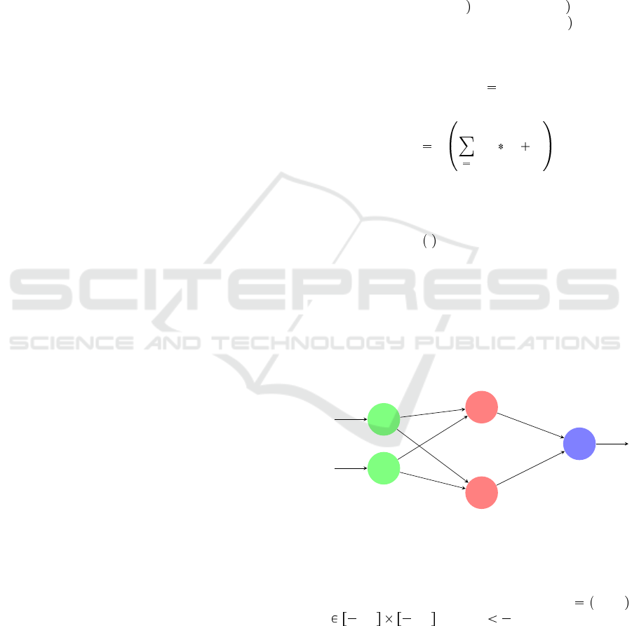
x
1
x
2
H
1
H
2
y
1
1
1
-1
1
-1
Figure 1: Example of neural network.
Fig.1 illustrates a simple example of feed-forward
with only one hidden layer. Hence, the NNV prob-
lem in this figure, consists in answering some ques-
tions such as: Is there an input vector ~x x
1
,x
2
2,2 2,2 where y 5 ?
Dynamic and Scalable Deep Neural Network Verification Algorithm
1123

2.2 General Neural Networks
Verification Problem
Given a deep neural network N : x y, a set of prop-
erties P covering the inputs and a set Q covering the
outputs, the NNV problem is to answer the follow-
ing question: Is there an input x resulting an output
y N x , verifying P and failing Q ?
In the rest of our paper, we consider:
• P x represents the constraints fixed on inputs
(for example, input should belongs a predefined
range).
• Q x represents constraints fixed on outputs.
For sake of clarity, we take the example of Fig.1
to illustrate P and Q that can be written as follows:
• P x x
1
2 x
1
2 x
2
2 x
2
2
• Q y y 5
3 RELATED WORK
The robustness of decision-making functions in un-
certain environment is an important research domain.
In the automotive context, the perturbation of environ-
ment can be caused by the failure of perception sen-
sors. So to ensure operational safety and road safety,
it is crucial to assure the robustness of these systems
faced sensor uncertainty. Recently, several research
studies have demonstrated the sensitivity of the neu-
ral network against certain attacks. In this section, we
present a state of the art of approaches proposed to
verify a Neural Network, i.e evaluate the robustness
of Neural Network in uncertain environment.
The proposed approaches can be grouped accord-
ing to the formulation of the problem. We focus on the
three following formulations: feasibility problem for-
mulation, reachability problem formulation and opti-
mization problem formulation.
3.1 Feasibility Problem Formulation
The principle of this approach (formulation) consists
in converting the Neural Network to a feasibility prob-
lem for the existence of an counter-example. The al-
gorithm, in this case, returns an information in the
following form: ”a counter-example is found” or ”no
counter-example is found”.
The verification process includes a set of mini-
tasks:
1. Convert the neural network to a set of equations
using the relationship between neurons of succes-
sive network layers.
2. Add an infeasibility constraint (example: Q y ,
where is the logical negation operator).
3. Search of a counter-example:
• If a counter-example is found , the initial prob-
lem is called non-feasible.
• If no counter-example is found, the initial prob-
lem is called feasible.
As described in 2.1, a Neural Network includes
activation functions which are generally non-linear
(e.g., tanh x , Sigmo
¨
ıde x
1
1 e
x
and ReLU x
max x, 0 ). This non linearity makes the complexity
of the problem NP-Hard. In this case, the contribution
of different articles/papers in the literature consists in
proposing a solution to linearize activation functions
(see Table 1).
In (Katz et al., 2017), authors propose to adapt
the simplex algorithm, a standard algorithm for solv-
ing linear programming, to non-linear activation func-
tions, specifically to support the ReLU function
(ReLU for ” Rectified Linear Unit”). The algorithm is
called Reluplex, i.e. ReLU with the simplex method.
Reluplex uses the simplex algorithm to search a feasi-
ble activation pattern that leads to an in-feasible out-
put. The principle of Reluplex is to solve a system of
equation from an initial assignment. At each iteration,
the algorithms attempts to correct certain constraints
violation. In fact, from one iteration to another, vari-
able assignment can violate constraints.
In (Bunel et al., 2018), the authors propose
PLANET (for ”a Piece-wise LineAr feed-forward
NEural network verification Tool”). It consists first in
replacing the non-linear functions of the Neural Net-
work by a set of linear equations. Then, the algo-
rithm tries to find a solution for the resulting system
of equations.
3.2 Reachability Problem Formulation
The reachability problem can be formulated as fol-
lows: given a computational system with a set of al-
lowed rules, decide whether a certain state of a system
is reachable from a given initial state of the system.
The process of verification includes three main steps:
1. Compute the input set X defined as all possible
inputs that system can takes as input.
2. Compute the output reachable set Y defined as:
Y y y N x ,x X , where N is the Neural
Network function.
ICAART 2021 - 13th International Conference on Agents and Artificial Intelligence
1124

Table 1: Summary of research work related to NNV.
Reference Principle Year
Feasibility formulation
(Katz et al., 2017) Using the simplex algorithm 2017
(Ehlers, 2017) Linearization of the nonlinear functions 2017
(Bunel et al., 2018) Using the heuristic Branch & Bound 2018
Reachability formulation
(Xiang et al., 2018) Approximation of the reachability set by a sensitivity study 2018
(Gehr et al., 2018) Over-approximation of the reachability set using the abstract interpretation 2018
(Xiang et al., 2018) Exact calculation of all reachability 2018
Approximation formulation
(Lomuscio and Maganti, 2017) Resolution of a linear program by Gurobi algorithm 2017
(Tjeng et al., 2019) Search of the maximum disturbance to distort Neural Network 2019
(Dvijotham et al., 2018) Approximation using Lagrangian relaxations 2018
(Wong and Kolter, 2018) Approximation using convex relaxation 2018
(Raghunathan et al., 2018) Convex optimization by the positive semi-definite method 2018
3. Check if Y satisfies the constraints Q (constraints
fixed on outputs).
Moreover, the determination of the reachable set Y
can be taxonomized into two main categories:
1. Exact (optimal) approaches: to model inputs, no
assumption is considered. This type of approach
look for the exact set of reachable output.
2. Approximate (near-optimal) approaches: to
model inputs, assumptions are considered. The
input set is generally over approximated using
standard geometric shapes. In fact, the reachable
set is not the exact output set but a over approxi-
mation.
In (Xiang et al., 2018), only neural network with
ReLU activation function can be considered. To de-
termine the exact reachable set, the authors assume
that the input and output are represented by the union
set of polytopes. Moreover, any over-approximation
is applied. Hence, the number of polytopes grows ex-
ponentially with each layer.
In (Gehr et al., 2018), the authors propose ”Ab-
stract Interpretation for Artificial Intelligence (AI2)”
technique. It consists in over-approximating inputs
using geometric shapes namely zonohedron. Then,
each Neural Network layer is converted to a equiv-
alent abstract layer. Finally, the input shape evolves
through the layers of the network. The, output shape
is called the reachable set.
3.3 Optimization Problem Formulation
The optimization problem consists in converting the
Neural Network to a set of conjunction or dis-junction
of linear properties. Given the example of a ”Fully-
connected” layer, it can be represented by a chain of
conjunctions as follows. As notation, the variables x
i
represents the output vector of layer i. The relation-
ship between successive layers (x
i 1
and x
i
) can be
encoded by the constraint C
i
as follows:
C
i
x
j
i
w
j
i
x
i 1
b
j
i
where w
i
j
is the j
th
column of w
i
, w is the weight ma-
trix and b is the bias matrix. After encoding all lay-
ers, the Neural Network is represented by the junc-
tion of all conjunctions. Several solutions have been
proposed to solve the previously obtained system,
and can be grouped into two groups: primal problem
based and dual problem based.
Regarding primal-based formulation, this type of
approaches consists in solving directly system equa-
tions using linear programming. In (Lomuscio and
Maganti, 2017) authors convert the Neural Network
to a set of constraints. Then the algorithm Gurobi is
applied to find a solution. In (Tjeng et al., 2019), au-
thors seek the maximum perturbation to miss-classify
the Neural Network using the Mixed-integer linear
programming (MILP).
Regarding dual-based approaches, the idea is to
use relaxations (approximations) of linear equations
to solve the optimization problem. In (Dvijotham
et al., 2018), authors propose the use of Lagrangian
relaxation to approximate bounds of neuron values. In
(Wong and Kolter, 2018), to estimate bounds, authors
use convex relaxations. The authors of (Raghunathan
et al., 2018) propose the use of positive semi-definite
optimization to approximate bounds.
Dynamic and Scalable Deep Neural Network Verification Algorithm
1125

4 THE PROPOSED APPROACH
In this section we describe the proposed adaptive and
scalable neural network verification algorithm. Table
2 defines the NNV parameters used to formulate the
problem of Figure 1. We consider a neural network as
an input. It is encoded as series of data inputs ranging
from lower to upper bounds. Moreover, neural net-
work nodes have activation functions applied at the
output of an artificial neural node in order to trans-
form the incoming flow into another domain. It is
worth mentioning here that the considered activation
function is the ReLU function. For sake of clarity,
ReLU function is given by:
ReLU X max X ; 0 (2)
where X represents the incoming flow at that artificial
node.
ReLU is a non-linear activation function. There-
fore, we propose to consider the bigM technique as
an automated encoder that linearizes the hidden con-
straint. It is a mixed integer linear programming trans-
formation that exactly transforms non-linear con-
straints into linear inequalities. More details on bigM
are given in the sequel.
4.1 Generalized Big-M Approach in
Deep Neural Networks
To solve the NNV problem, we propose a general
mathematical formulation to handle with various deep
neural networks. In other words, we consider differ-
ent neural networks sizes with large data input, sev-
eral hidden layers, and outputs representing the deci-
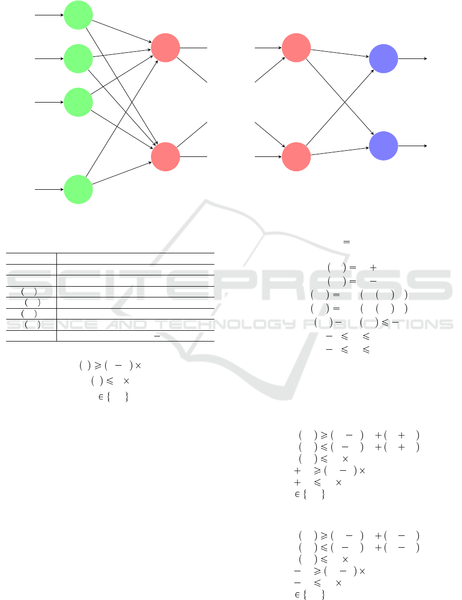
sion. In Fig. 2, and for sake of clarity, we depict a
typical example to be considered in our modelling.
Therefore, we consider a neural network with m
layers noted by L
1
,L
2
,...,L
m
. In each layer, we
consider n neurons represented by nodes in Fig.2.
There exists an arc i, j between each neuron i in a
layer L
s
and j in a different layer L
t
(s t). This arc is
weighted by w
i j
as depicted by Fig.2. Moreover, for
each neuron j (node in the graph of Fig.2), we con-
sider two main variables a
in
j and a
out
j given by
the following:
1. if j L
1
, hence we have the two following inputs:
• a
in
j x
j
• a
out
j x
j
2. if j L
k
where 2 k m 1, hence we have:
• a
in
j
i Γ j
w
i j
a
out
i
• a
out
j max a
in
j ;0
3. if j L
m
(last layer in our neural network):
• a
in
j
i Γ j
w
i j
a
out
i
• a
out
j max a
in
j ;0 : not concerned in our
scenarios.
where Γ j indicates the set of predecessor nodes of
j in the considered neural network.
According to the previous modelling, we propose
in the following the final mathematical model that will
serve to identify if our system has at least one solution
or not:
maxZ Constant
S.T. :
j L
1
:
a
in
j x
j
a
out
j x
j
j L
k
2 k m 1 :
a
in
j
i Γ j
w
i j
a
out
i
a
out
j max a
in
j ;0
j L
m
:
a
in
j
i Γ j
w
i j
a
out
i
a
in
j
i Γ j
w
i j
a
out
i β
a
0
x
j
b
0
(3)
where a
0
and b
0
are real inputs (a
0
,b
0
R) and β R
is a parameter known before the optimization process.
Verifying the existence of any violation of the
mathematical formulation (3) is equivalent to solve
this system of non linear inequalities and some linear
equalities and hence verifying if certain constraints
are violated by others or not.
In system (3), inequalities using to determine the
maximum between 0 and a
in
j (for a given neuron
j) are non-linear and necessitate to be linearized to
facilitate solving the model in negligible times.
In the sequel, we propose a linearization approach
based on Big-M technique to totally eliminate non-
linear equalities in the mathematical formulation (3).
We consider, for instance, the following non-linear
equality (for a given j):
a
out
j max a
in
j ;0 (4)
We introduce a new binary variable θ 0, 1 to
discuss the different cases that can be resulted from
(4). In fact, we consider:
a
out
j
a
in
j , if a
in
j 0
0, else
Hence, we propose:
a
out
j θ 1 M a
in
j (5)
a
out
j 1 θ M a
in
j (6)
a
out
j θ M (7)
ICAART 2021 - 13th International Conference on Agents and Artificial Intelligence
1126

.
.
.
.
.
.
.
.
.
.
.
.
x
1
x
2
x
3
x
n
H
1
1
H
n
1
H
1
m
H
n
m
y
1
y
m
w
11
w
21
w
31
w
n1
w
11
w
1m
w
n1
w
nm
Input
layer
Hidden
layer
Hidden
layer
Output
layer
.. .
Figure 2: Example of neural network.
Table 2: Neural Network Verification Problem Notation.
Parameters Definition
x
1
input 1 in L
1
x
2
input 2 in L
1
a
in
H
1
input to the H
1
a
out
H
1
non linear function of a
in
(output of H
1
)
a
in
H
2
input to the H
2
a
out
H
2
non linear function of a
in
(output of H
2
)
β a parameter with a value of 5
a
in
j θ 1 M (8)
a
in
j θ M (9)
θ 0,1 (10)
Using the formulations (5) to (9), one can verify, ac-
cording to the values of θ, that we can attend the same
results than those of equation (4).
For sake of clarity, we propose to discuss deeply
the example of Figure 1, and hence we apply the result
of the proposed and generalized mathematical formu-
lation (3) on this example (see Figure 1).
4.2 BigM Approach: Application on
Example of Figure 1
We consider the example of Fig.1, the Neural Net-
work consists of three layers L
1
,L
2
,L
3
, with one node
in the L
3
(output layer). Table 2 is summarizing the
different parameters of the example of Fig.1.
The Big-M approach for the example of Fig.1 can be
formulated as follows (according to system (3)):
max Z Constant (11)
Sub ject to
a
in
H
1
x
1
x
2
(12)
a
in
H
2
x
1
x
2
(13)
a
out
H
1
max a
in
H
1
,0 (14)
a
out
H
2
max a
in
H
2
,0 (15)
a
out
H
1
a
out
H
2
5 (16)
2 x
1
2 (17)
2 x
2
2 (18)
This formulation (from (12) to (18)) is non linear as it
contains at least two non-linear ReLU activation func-
tions or equations given by (14) and (15). Therefore,
we propose to linearize this model to obtain a solution
if exists. Hence, equation (14) will be formulated as
follows.
a
out
H
1
θ
1
1 M x
1
x
2
a
out
H
1
1 θ
1
M x
1
x
2
a
out
H
1
θ
1
M
x
1
x
2
θ
1
1 M
x
1
x
2
θ
1
M
θ
1
0,1
(19)
Similarly, equation (15) is linearized as the following
a
out
H
2
θ
2
1 M x
1
x
2
a
out
H
2
1 θ
2
M x
1
x
2
a
out
H
2
θ
2
M
x
1
x
2
θ
2
1 M
x
1
x
2
θ
2
M
θ
2
0,1
(20)
Dynamic and Scalable Deep Neural Network Verification Algorithm
1127

Proposition 4.1. The mathematical formulation con-
cerning equations (inequalities) from (12) to (18) has
no solution in the defined domain.
Proof. We start the proof using the following mathe-
matical formulation (after the proposed linearization),
in which we substitute a
in
, and b
in
by x
1
x
2
and
x
1
x
2
respectively. We obtain:
maxZ Constant
S.T. :
a
out
H
1
θ
1
1 M x
1
x
2
a
out
H
1
θ
1
M
x
1
x
2
θ
1
1 M
x
1
x
2
θ
1
M
a
out
H
2
θ
2
1 M x
1
x
2
a
out
H
2
θ
2
M
x
1
x
2
θ
2
1 M
x
1
x
2
θ
2
M
a
out
H
1
a
out
H
2
5
2 x
1
2
2 x
2
2
(21)
We suppose that θ
1
θ
2
. If we consider the differ-
ence between the first inequality of the model (21)
and the fifth inequality of the same model, then we
obtain:
a
out
H
1
a
out
H
2
2x
2
(22)
At the same time, we also considered:
a
out
H
1
a
out
H
2
5 (23)
Hence, the addition (22)+(23) will lead to:
x
2
5
2
(24)
The result (24) contradicts the domain of x
2
provided
by (18). Hence, there is no solution for this system in
the respective domains of x
1
and x
2
.
5 PERFORMANCE EVALUATION
5.1 Neural Network Configuration
Setting
The final system of equations (3) is implemented us-
ing IBM CPLEX optimization tool and considering a
constant objective function to optimize. We have con-
sidered a feed-forward neural network architecture.
We show in Table 3 hereafter the used simulation pa-
rameters.
Table 3: Neural Network Configuration Setting.
Simulation Parameters Values
m from 50 to 100 which models most
of the neural networks (Carlini and
Wagner, 2018)
n 50 and 100 neurons
Type Fully connected
M or Big M infinity
θ Binary decision variable (0 or 1)
x
j
j 1,. .. ,n normalized and scaled data inputs
y
j
classes or predicted values. We
specify single and multi output neu-
rons
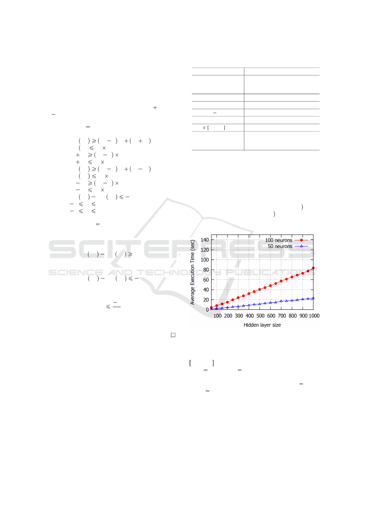
5.2 Impact of n and m on Convergence
Time
In this section, we investigate the impact of varying
the input size n in the verification optimization in-
stances. Hence, we address two scenarios: i a first
scenario of 50 input neurons and ii a second scenario
of 100 input neurons.
Figure 3: Execution time of different input sizes.
Figure 3 depicts the necessary convergence time
of our approach for a hidden layer size (m) in the
20,1000 interval. We considered the two scenarios
of n 50 and n 100 neurons to illustrate the
negligible necessary execution time which approx-
imates 80 seconds in the worst case (m 1000,
and n 100) to reach the optimal solution. This is
due to the efficiency of our complete mathematical
formulation to converge rapidly to optimal solutions
even for large problem instances. Hence, we show the
feasibility of our Big-M based verification algorithm
for the considered scenarios and illustrate clearly the
scalability of this method. Indeed, our mathematical
formulation is linear and its resolution is based on a
ICAART 2021 - 13th International Conference on Agents and Artificial Intelligence
1128

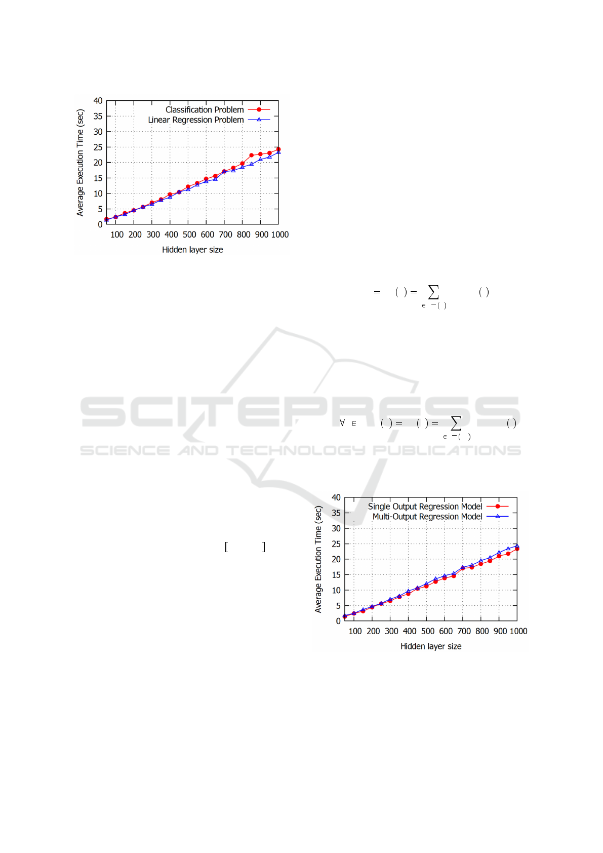
Figure 4: Execution time of linear regression and classifica-
tion problems.
simple relaxation of the ReLU equalities leading to
deeply simplifying the initial considered problem.
In the following, and to highlight the efficiency of
our approach, we consider two verification problems
based on linear regression and classification.
5.3 Linear Regression and
Classification Problems Verification
We consider linear regression and classification mod-
els (the set of problem constraints) in order to evaluate
the time complexity of the proposed Big-M based ver-
ification algorithm. We set in both problems 50 neu-
ron processors as the input size (it represents a typical
configuration parameter).
We run 100 times the two scenarios using our Big-
M based approach and take the average value of the
necessary execution time (in seconds) to obtain the
optimal solutions. Figure 4 depicts the same evolution
of the convergence time for the two problems when
the number of hidden layers is in the 100, 800 inter-
val. For hidden layers with size between 800 and 900
neurons, we can observe a slight difference in favor of
the linear regression problem. Indeed, this small dif-
ference is due to considering more binary variables in
the formulation of the classification problem, which
necessitates more time to converge to the optimal so-
lution. For more than 900 hidden layer neurons, the
average execution time for the classification problem
converges to the average necessary time of the lin-
ear regression problem, which confirms the efficiency
and the scalability of our proposed Big-M-based ap-
proach to the optimal solution even for large instances
(the worst case in Figure 4 converges in less than 25
seconds).
5.4 Single-output and Multi-output
Verification Scenarios
To extend the illustration and the efficiency of our ap-
proach, we propose to consider two new scenarios ad-
dressing a neural network with a single output, and
another scenario with multiple output. The verifica-
tion of these scenarios using our approach consists in
modifying the two last inequalities of the mathemati-
cal formulation (3).
• Single Verification Scenario. In this scenario,
our neural network outputs a single value. The
verification of the model is realized using a single
output constraint (last constraint of (3) adapted to
this scenario). It is formulated as follows:
y a
in
o
i Γ o
w
i,o
a
out
i (25)
Where o is the single output neuron at the output
layer.
• Multi-output Verification Scenario. In this sce-
nario, the considered neural network outputs a
multi-output. The verification problem consists of
multi-output constraints. Each output constraint
may represent a verification problem instance. It
is formulated as follows:
j L
m
, y j a
in
j
i Γ o
j
w
i,o
j
a
out
i
(26)
Where o
j
is the j
th
output neuron at the output
layer.
Figure 5: Execution time of single and multi-output prob-
lem instances.
Figure 5 depicts the behavior of the proposed Big-M
optimisation problem according to the above scenar-
ios. It shows that adding extra output constraints re-
quires a slight and negligible (less than 3 seconds in
Dynamic and Scalable Deep Neural Network Verification Algorithm
1129

the worst case) augmentation of execution time which
proves the feasibility of the algorithm in complex sce-
narios.
6 CONCLUSION AND
PERSPECTIVES
In this paper, we examined the safety of Neural Net-
work against input perturbations i.e in an uncertain
environment. Our challenge was to verify neural net-
work output according to input range and provide a
formal guarantees about its behavior. Hence, our con-
tribution to the formulation of the verification prob-
lem is based on linear programming technique. We
proposed an exact mathematical formulation and then
eliminated the non-linearities by encoding them with
the help of binary variables. In the numerical eval-
uation, different scenarios are discussed, and results
show that our approach is feasible, in terms of con-
vergence time, and scalable even for large neural net-
works.
Our approach considered only neural network
with ReLU activation functions. In future work, we
plan to extend our study to other activation functions,
such as Tanh, Sigmo
¨
ıde, etc. Moreover, we plan to
validate our proposed approach on real use cases such
as image classification, self driving, etc.
REFERENCES
Bunel, R., Turkaslan, I., Torr, P. H., Kohli, P., and Kumar,
M. P. (2018). A unified view of piecewise linear neu-
ral network verification. In Proceedings of the 32Nd
International Conference on Neural Information Pro-
cessing Systems, NIPS’18, pages 4795–4804, USA.
Curran Associates Inc.
Carlini, N. and Wagner, D. (2018). Audio adversarial ex-
amples: Targeted attacks on speech-to-text. In 2018
IEEE Security and Privacy Workshops (SPW), pages
1–7.
Dvijotham, K., Stanforth, R., Gowal, S., Mann, T. A., and
Kohli, P. (2018). A dual approach to scalable verifica-
tion of deep networks. In Proceedings of the Thirty-
Fourth Conference on Uncertainty in Artificial Intelli-
gence, UAI 2018, Monterey, California, USA, August
6-10, 2018, pages 550–559.
Ehlers, R. (2017). Formal verification of piece-
wise linear feed-forward neural networks. CoRR,
abs/1705.01320.
Gehr, T., Mirman, M., Drachsler-Cohen, D., Tsankov, P.,
Chaudhuri, S., and Vechev, M. (2018). Ai 2: Safety
and robustness certification of neural networks with
abstract interpretation. In Security and Privacy (SP),
2018 IEEE Symposium on.
Jmila, H., Khedher, M. I., Blanc, G., and El-Yacoubi, M. A.
(2019). Siamese network based feature learning for
improved intrusion detection. In Gedeon, T., Wong,
K. W., and Lee, M., editors, Neural Information
Processing - 26th International Conference, ICONIP
2019, Sydney, NSW, Australia, December 12-15, 2019,
Proceedings, Part I, volume 11953 of Lecture Notes in
Computer Science, pages 377–389. Springer.
Katz, G., Barrett, C. W., Dill, D. L., Julian, K., and Kochen-
derfer, M. J. (2017). Reluplex: An efficient SMT
solver for verifying deep neural networks. In Com-
puter Aided Verification - 29th International Confer-
ence, CAV 2017, Heidelberg, Germany, July 24-28,
2017, Proceedings, Part I, pages 97–117.
Khedher, M. I., Jmila, H., and Yacoubi, M. A. E. (2018).
Fusion of interest point/image based descriptors for
efficient person re-identification. In 2018 Interna-
tional Joint Conference on Neural Networks (IJCNN),
pages 1–7.
Lomuscio, A. and Maganti, L. (2017). An approach to
reachability analysis for feed-forward relu neural net-
works. CoRR, abs/1706.07351.
Raghunathan, A., Steinhardt, J., and Liang, P. (2018).
Certified defenses against adversarial examples. In
6th International Conference on Learning Represen-
tations, ICLR 2018, Vancouver, BC, Canada, April 30
- May 3, 2018, Conference Track Proceedings. Open-
Review.net.
Tjeng, V., Xiao, K. Y., and Tedrake, R. (2019). Evaluating
robustness of neural networks with mixed integer pro-
gramming. In 7th International Conference on Learn-
ing Representations, ICLR 2019, New Orleans, LA,
USA, May 6-9, 2019. OpenReview.net.
Wong, E. and Kolter, J. Z. (2018). Provable defenses against
adversarial examples via the convex outer adversar-
ial polytope. In Dy, J. G. and Krause, A., editors,
Proceedings of the 35th International Conference on
Machine Learning, ICML 2018, Stockholmsm
¨
assan,
Stockholm, Sweden, July 10-15, 2018, volume 80 of
Proceedings of Machine Learning Research, pages
5283–5292. PMLR.
Xiang, W., Tran, H., and Johnson, T. T. (2018). Output
reachable set estimation and verification for multi-
layer neural networks. IEEE Transactions on Neural
Networks and Learning Systems, 29(11):5777–5783.
Xiang, W., Tran, H.-D., and Johnson, T. T. (2018). Reach-
able set computation and safety verification for neural
networks with relu activations. In Submission.
ICAART 2021 - 13th International Conference on Agents and Artificial Intelligence
1130