Tourism Forecast with Weather, Event, and Cross-industry Data

Simone Lionetti

1 a

, Daniel Pf

afﬂi

1 b

, Marc Pouly

1 c

, Tim Vor Der Br

uck

1 d

and Philipp Wegelin

2 e

School of Computer Science and Information Technology, Lucerne University of Applied Sciences and Arts, Suurstofﬁ 1,

6343 Rotkreuz, Switzerland

School of Business, Lucerne University of Applied Sciences and Arts, Zentralstr. 9, 6002 Lucerne, Switzerland

Keywords:

Forecasting, Tourism, Machine Learning, Deep Learning, Feature Importance, Dataset.

Abstract:

The ability to make accurate forecasts on the number of customers is a pre-requisite for efﬁcient planning and

use of resources in various industries. It also contributes to global challenges of society such as food waste.

Tourism is a domain particularly focussed on short-term forecasting for which the existing literature suggests

that calendar and weather data are the most important sources for accurate prediction. We collected and make

available a dataset with visitor counts over ten years from four different businesses representative for the

tourism sector in Switzerland, along with nearly a thousand features comprising weather, calendar, event and

lag information. Evaluation of a plethora of machine learning models revealed that even very advanced deep

learning models as well as industry benchmarks show performance at most on a par with simple (piecewise)

linear models. Notwithstanding the fact that weather and event features are relevant, contrary to expectations,

they proved insufﬁcient for high-quality forecasting. Moreover, and again in contradiction to the existing

literature, performance could not be improved by including cross-industry data.

1 INTRODUCTION

Substantial short-term demand ﬂuctuations are com-

mon in the tourism industry. Therefore, tourism com-

panies such as accommodation, transportation, cater-

ing, and leisure facilities have a vital interest in pre-

cise forecasts of the number of customers. Such fore-

casts fulﬁll at least three purposes. First, they allow

efﬁcient planning and use of resources, thereby pre-

venting misallocation, which may manifest as either

shortage or waste. Shortage can lead to overuse (ex-

hausted staff) and queuing (dissatisﬁed customers).

Waste occurs when unused services (empty bus rides,

unconsumed meals) expire worthless according to the

uno actu or no-stock-keeping principle. Second, pre-

cise customer forecasts allow companies to engage

in dynamic pricing and revenue management. Third,

forecasts can be used to inform potential customers,

for instance about crowding. Precise tourism fore-

casts thus provide immediate economic, societal, and

https://orcid.org/0000-0001-7305-8957

https://orcid.org/0000-0002-2957-5735

https://orcid.org/0000-0002-9520-4799

https://orcid.org/0000-0003-1732-6392

https://orcid.org/0000-0002-7231-0302

environmental beneﬁts.

A number of companies in the tourism industry

like some hotels and airports can rely on advanced

booking for customer forecasts. To date, most other

tourism businesses base their forecasts on the intuitive

expertise of responsible managers, possibly comple-

mented with simple statistics such as some lagged

number of customers or an average over a certain time

period. One reason for this is that many tourism com-

panies are Small and Medium Enterprises (SMEs)

that lack ﬁnancial resources and knowhow to imple-

ment sophisticated forecasting methods. While the

expertise is undoubtedly powerful, the use of statis-

tical methods can signiﬁcantly improve demand fore-

casts and related decision making (Armstrong, 2001;

Hu et al., 2004). As competition in the tourism in-

dustry grows and additional challenges appear (e.g.

climate change or the Covid19 crisis), the industry

is pushed more than ever to optimize operations and

business models.

Several previous studies have dealt with forecast-

ing daily customer numbers in the tourism indus-

try, and have found signiﬁcant explanatory power

of weather and event features. A pioneering work

(Dwyer, 1988) dealt with an urban recreation site in

the Chicago area, stressing the importance of weather,

Lionetti, S., Pfäfﬂi, D., Pouly, M., vor der Brück, T. and Wegelin, P.

Tourism Forecast with Weather, Event, and Cross-industry Data.

DOI: 10.5220/0010323010971104

In Proceedings of the 13th International Conference on Agents and Artiﬁcial Intelligence (ICAART 2021) - Volume 2, pages 1097-1104

ISBN: 978-989-758-484-8

1097

season, and day of the week. (Brandenburg and Arn-

berger, 2001) addressed forecasting for a national

park near Vienna, highlighting the importance of cal-

endar effects and temperature. Ski destinations in

the state of Michigan were considered in (Shih et al.,

2009; Shih and Nicholls, 2011), where temperature,

snow depth, holidays, and weekends were found to be

relevant. Other variables known to have an effect on

tourism include income, price, travel expenses, and

trends (Song et al., 2003).

It is to be noted that there is no common agree-

ment on the best quantity to measure the performance

of forecasting models in tourism. A possible reason

for this is that time series for different businesses have

signiﬁcantly different properties such as mean value,

variance, seasonality, and number of zeros. Another

factor may be that the economic cost of errors highly

depends on the speciﬁc company under examination.

Because of this, extra care is needed when compar-

ing performance on different time series or evaluating

current practices.

In recent years, the state-of-the-art in forecasting

has seen a gradual shift from linear models and Ex-

ponential Smoothing (ES) to more sophisticated Ma-

chine Learning (ML) techniques. The most popu-

lar approaches include gradient boosting (Makridakis

et al., 2020b), Recurrent Neural Networks (RNNs)

such as DeepAR (Salinas et al., 2020), and Deep

Learning (DL) models based on attention (Lim et al.,

2019; Zhou et al., 2020), but also Prophet (Taylor

and Letham, 2018), a model based on time series sea-

sonal decomposition with changepoints and learnable

weights for holidays, which has emerged as a quasi-

industrial standard.

Massive efforts have also been conducted to un-

derstand the practical advantages of different ap-

proaches. The M4 competition considered 100,000

time series categorized in six domains and six reso-

lutions. 61 forecasting strategies submitted for M4

were analyzed in (Makridakis et al., 2020a). The top

performing method was a hybrid algorithm that com-

bined ES and RNNs with joint optimization (Smyl,

2020). A major result of M4 was the conclusion that

cross-series information is highly beneﬁcial. The suc-

cessor competition M5 focussed on 48,840 time se-

ries for item sales of stores in various locations with

a 28-day forecasting horizon. M5 included explana-

tory variables such as calendar effects, selling prices,

and promotion events. Results were summarized in

(Makridakis et al., 2020b). The best performance was

achieved by training 220 LightGBM models and se-

lecting an ensemble of 6 of them for each series. Once

again, models that used cross-learning from multiple

series performed signiﬁcantly better than the ones that

did not. Moreover, simple ML methods were found

to be superior to more sophisticated ones. In the SME

landscape, however, it is unfeasible to gather such a

large database to train robust forecast models.

In this paper, we consider four diverse companies

which operate in the tourism sector and are located in

the same region of Switzerland. These destinations

are of international relevance and great economic in-

terest given the importance of tourism in this coun-

try. More precisely, we address one-day-ahead fore-

casting of the total number of daily customers for the

ten years from 2007 to 2016. The dataset is anno-

tated with events and weather forecast variables, and

is made publicly available as part of this contribu-

tion. We claim that in this context, notwithstanding

the fact that date, event, and weather features are rel-

evant, contrary to expectations, they are not sufﬁcient

for high-quality forecasting. Moreover, we also argue

that in the case at hand there is no signiﬁcant bene-

ﬁt from a joint forecasting of multiple time series of

similar nature.

The paper is structured as follows. In section 2

we describe the collected dataset, its main features

and how to access it publicly. Section 3 sets up the

evaluation procedure, a simple approximation of the

underlying stochastic process, and the ML models we

explored. In section 4 we present selected numerical

results and illustrate how they support our claims. We

then conclude in section 5 with more precise state-

ments and an outlook on further steps that are needed

to complete our investigation.

2 DATASET

In this section we present a novel forecasting dataset

for tourism, which is made publicly available

as part

of this contribution (Pf

afﬂi et al., 2020).

2.1 Target Variables

The four Swiss companies we consider consist of one

accommodation, two transportation, and one indoor

leisure businesses, all located in the same touristic re-

gion. The customer volume data has daily resolution

and features at worst minor interruptions of a few days

over a common period of ten years starting in 2007

and ending in 2016. The missing values for one trans-

portation and the indoor leisure company are masked,

and the masks are available as indicator variables. For

all evaluations reported in this work, forecasts on the

few missing values are ignored.

http://dx.doi.org/10.5281/zenodo.4133644

ICAART 2021 - 13th International Conference on Agents and Artiﬁcial Intelligence

1098

Table 1: Statistical ﬁgures of the four individual datasets

and the combined dataset (removing duplicate features).

Company Features Target mean Target std

Accommodation 615 63 24

Transport 1 615 1106 937

Transport 2 468 2669 1654

Indoor leisure 430 1121 461

Combined 932 - -

2.2 Feature Variables

We include date variables for calendar effects, such as

e.g. the day of the week. Event data thought to be rel-

evant for understanding customer behavior includes

public and school holidays, free-time regional events,

as well as promotions or revisions for the facilities

under examination. The weather forecast features are

provided by the Federal Ofﬁce of Meteorology and

Climatology (MeteoSwiss), and encode extended in-

formation about conditions in the locations of the four

businesses and neighboring regions. They consist

of data for temperature, sunshine, precipitation, and

wind, forecasted up to 3 days in advance. The dataset

thus constructed contains 562 variables both numer-

ical and categorical. Note that the weather forecast

model is updated regularly, and therefore many fea-

tures do not cover the entire period. Transformed into

a vector space model by means of one-hot encoding,

we count 932 features, four target and two mask vari-

ables. The number of features semantically associated

to each company after the transformation is summa-

rized in table 1; additional information can be found

in the download documentation.

In all experiments reported in this work, we ex-

plicitly include the targets with lags from 1 to 7 days

among features. We note that the number of features

is relatively large compared to the amount of avail-

able data to ﬁt, which consists of a single number per

company for each of the 3653 days in the years 2007–

2016.

2.3 Publication

In the published version of the dataset, feature names

are replaced with pseudonyms but descriptions are

given to identify feature groups with similar meaning.

The content available for download consists of

• data.csv, CSV format, 11.3 MB, 3654 rows and

562 columns with the time series data;

• data-description.csv, CSV format, 36 KB,

563 rows and 12 columns with feature name and

short description, minimal statistics for cross-

checking, and indicator variables that specify to

which single-company datasets a feature belongs.

3 METHODS

3.1 Evaluation

In order to assess ﬂuctuations of performance scores

due to ﬁnite sample size and take full temporal depen-

dence into account, we rely on sequential validation.

More precisely, we create folds with n consecutive

years for training and the following year for evalua-

tion. We work with whole years to mitigate the inﬂu-

ence of seasonality on the scores. We start from n = 4

to guarantee a sufﬁcient amount of training data. The

ﬁve folds with n = 4 to 8 are used for cross-validation

and the one with n = 9 is kept out for testing.

As mentioned in section 1, the metric to evaluate

the performance of predictions is not uniquely deﬁned

either by the problem or by convention. Given our

time series contain a signiﬁcant amount of small inte-

ger values, including zeros which may be accidental

or systematic, we refrain from using precision errors.

Instead, we compare results using the coefﬁcient of

determination R

. We observe that, up to rescaling

and shift, this metric is equivalent to Mean Squared

Error (MSE). When the evaluation time range is small

compared to the span of past values, R

is also approx-

imately equivalent to (Root) Mean Squared Scaled Er-

ror (Hyndman and Koehler, 2006).

3.2 Theoretical Bound

Customer turnout is the result of many binary (almost)

individual decisions based on external conditions. As-

suming these decisions obeys Bernoulli statistics, in

the limit of a large number of individuals N and small

turnout probability p, the outcome is described by a

Poisson distribution. On the one hand, potential cus-

tomers are represented by the local population and

travelling tourists, which is very high compared to

the turnout of all considered businesses on any given

day: the limit of N → ∞, p → 0 with constant λ = pN

seems justiﬁed. On the other hand, it is clear that the

decision process is not the same for every potential

customer, the assumption of independence is violated

by small groups, and saturation effects are ignored, so

the model is only an approximation of reality.

Based on these considerations, the observed time

series can be modelled as a Poisson process where the

probability to observe a number of customers k on a

speciﬁc day is given by

p(k|λ) =

−λ

, (1)

where λ is a function of the features. For a given λ, the

prediction that minimizes the squared error on a given

Tourism Forecast with Weather, Event, and Cross-industry Data

1099

day is the mean value of the distribution E[k|λ] = λ

and the expected squared error is E[(k − λ)

|λ] = λ.

In practice, even a posteriori when observed values

are known, we do not have access to the distribution

itself but only to a single sample. Using an improper

uninformative prior p(λ) = 1 over the whole allowed

range λ ∈ [0, +∞), we obtain p(k, λ) = p(k|λ). The

best guess described above then gives

E[(k − λ)

|k] =

+∞

dλ (k − λ)

p(k, λ)

+∞

dλ p(k, λ)

= k + 2. (2)

This result represents the minimum forecast variance

that is expected when the number of customers fol-

lows a Poisson distribution with a mean that can be

exactly predicted using features. It can be used to es-

tablish a benchmark performance in an idealized case.

3.3 Models

We introduce some baselines for comparison with

more sophisticated ML models, i.e. we evaluate mod-

els which always predict the same number of cus-

tomers as 1, 7, 364, or 365 days before the target and

take the best score as a naive baseline for each dataset.

Additionally, we follow the approach in section 3.2 to

obtain an estimate of performance in an optimal, ide-

alized scenario. Finally, we gather a benchmark for

an up-to-date industry-ready approach to time-series

forecasting using Prophet.

As a ﬁrst non-trivial ML approach, we consider

linear models ﬁt on a hand-crafted feature set. This

feature set only considers a subset of weather and

event features and is based on the existing literature

(see section 1) plus extensive interviews with industry

representatives. It includes interaction terms to take

into account that the effect of features may depend on

each other, for instance weather may have a different

impact on demand on weekdays compared to week-

ends. These interactions are constructed among date

features (days of the weeks and months), and between

date and weather features.

We then progressively move to more sophisticated

models using all features along with regularization

to control overﬁtting. We use MSE as loss function

throughout because of the arguments outlined in sec-

tion 3.1. Since it is difﬁcult to guess which represen-

tation of the exogenous features would give the best

results, pre-processing is kept to a minimum. More

speciﬁcally, all features are treated on the same level,

categorical variables are one-hot encoded, numeri-

cal ones are scaled between minimum and maximum

value or normalized using mean and variance where

appropriate, and no interaction terms are considered

in this phase.

The approaches evaluated include Lasso, Ridge,

and Gaussian process regression from scikit-learn

(Pedregosa et al., 2011), regression trees with gradi-

ent boosting from xgboost (Chen et al., 2015) and

lightgbm (Ke et al., 2017), simple dense multilayer

perceptrons, RNNs with LSTM and GRU units, and

RNNs with attention from tensorflow and keras

(Abadi et al., 2016). For Lasso and Ridge regression

we conducted a one-dimensional search over the regu-

larization parameter. For Gaussian process regression

we explored an RBF kernel with constant and white-

noise terms, and a dot kernel plus white noise. We

then performed a grid search to choose appropriate

hyper-parameters. The dot kernel performed consid-

erably better than the RBF kernel, but it was still not

competitive with the best models. The gradient boost-

ing family achieved a consistently good performance

across folds using default values, and since prelimi-

nary experiments with settings such as tree depth did

not improve scores signiﬁcantly we did not tune these

models any further. For the DL models, instead, we

considered simple architectures with up to 4 layers

and 512 units, we tried optimization with different

learning rates using gradient descent with momentum

and Adam, and we explored several values for L

, L

and dropout regularization terms. We also investi-

gated switching to Poisson log-likelihood as a loss,

and generating pseudo-data with Poisson ﬂuctuations

for each epoch as an additional form of regularization.

Since all options need to be evaluated for each of the

four datasets and 5 different folds, we did not conduct

a full grid search but limited ourselves to changing

one parameter at a time. Finally, since DL models

struggled to achieve consistently good scores across

all folds, we did not investigate even more complex

approaches such as DeepAR.

4 RESULTS

Table 2 and ﬁg. 1 summarize the results of the base-

line, the theoretical upper bound, the linear models

with hand-crafted feature sets, the Prophet benchmark

and the best approach among all others. The scores

for Prophet and the best ML approach are reported

for several feature sets: one using only the date of the

observation (“date only”), one which uses all features

available as described in section 2.2 (“all feaures”),

and one where weather variables are summarized with

a few numbers (“basic weather features”). The latter

is constructed by considering forecasts only one day

in advance and picking a single variable for each of

the four main parameters (temperature, precipitation,

sunshine/cloud cover, wind) for each location. This

ICAART 2021 - 13th International Conference on Agents and Artiﬁcial Intelligence

1100

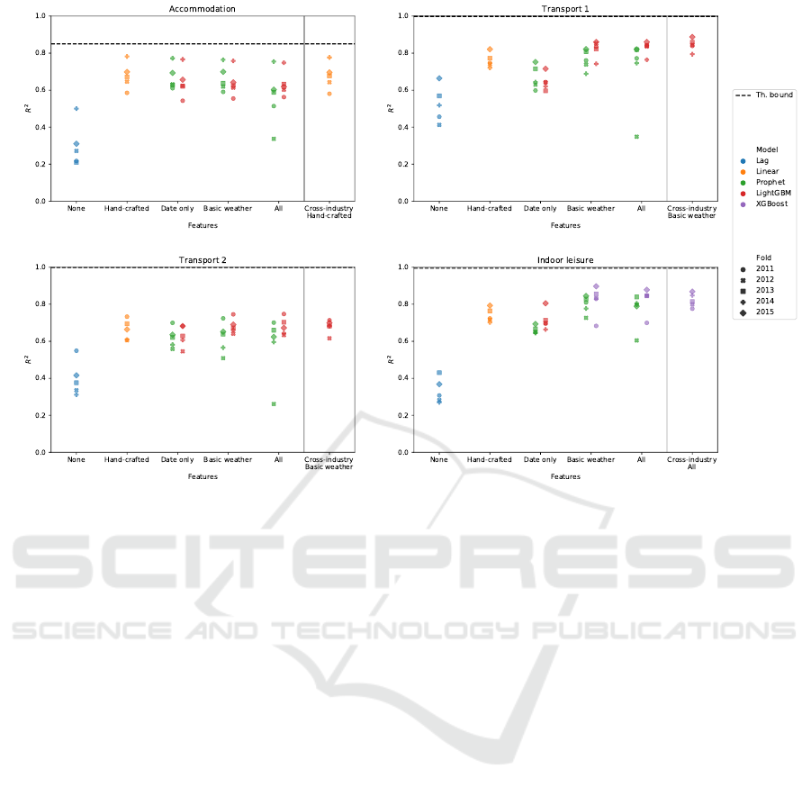
Figure 1: Comparison of the R

sequential validation scores for selected models and feature sets.

greatly reduces the number of features to around 100.

Note that 7 lagged target values are always included.

For each model and company, we report the mean R

and its standard deviation computed on the 5 folds.

For a meaningful comparison of scores obtained

using different feature sets, we also report the results

of hypothesis tests for selected pairs of results. More

precisely, we compare the sample score distributions

over the 5 folds to detect signiﬁcant differences of the

population means. These distributions are expected

to be signiﬁcantly non-gaussian at least when R

close to 1 and when there are outliers due to overﬁt-

ting. Nevertheless, due to the low number of sam-

ples, we decided to perform both a two-tailed paired

t-test and a two-tailed paired Wilcoxon signed-rank

test. We report the corresponding p-values and the

sign of the difference in table 2. The conclusions that

can be drawn with these two types of tests are some-

what different in strength but identical in content.

4.1 Model Comparison

We observe that the best scores are obtained by ei-

ther linear models or gradient boosting based on deci-

sion trees. They are signiﬁcantly better than the base-

lines and worse than the theoretical bounds. Prophet

is competitive with the best models if only the date

is used for prediction. Since in the accommodation

case including more features is not beneﬁcial as ex-

plained in section 4.2, Prophet remains on the same

level of the other best models for this company. Note

that depending on the exact feature set used, the per-

formance difference of linear models with interaction

terms, LightGBM, and XGBoost can be signiﬁcant.

DL models are not competitive in the settings we ex-

plored. In particular, we note that when all features

are used it is difﬁcult to introduce the right amount of

regularisation that allows learning but prevents over-

ﬁtting. As can be seen in the table, Prophet also some-

times struggles to deal with this issue.

4.2 Weather and Event Data

First we examine if weather and event data signiﬁ-

cantly improve predictions. To this end, we compare

the best model scores obtained using all features to

the ones obtained using only the date. Note that this

means that sometimes we compare different models

on different feature sets; however, conclusions are es-

sentially the same if any of the two models is chosen

for both feature sets. At the 95% conﬁdence level or

better, we can conﬁrm that for the indoor leisure struc-

ture and for the two transportation companies weather

and event data improves predictions. The accommo-

dation company, instead, shows a preference for re-

gression using only the date. While this could be a

Tourism Forecast with Weather, Event, and Cross-industry Data

1101

Table 2: R

validation scores for single-industry forecasting using different models and feature sets. The last two sections of

the table report p-values for testing the hypotheses described in section 4.2.

Company Accommodation Transport 1 Transport 2 Indoor leisure

Baselines

Lag baseline 0.301 ± 0.118 0.524 ± 0.099 0.398 ± 0.093 0.331 ± 0.067

Best naive lag 1 1 1 364

Theoretical bound 0.850 ± 0.021 0.9987 ± 0.0002 0.9988 ± 0.0001 0.9949 ± 0.0001

Date only

Prophet 0.667 ± 0.066 0.667 ± 0.064 0.613 ± 0.057 0.635 ± 0.021

This work 0.642 ± 0.081 0.643 ± 0.045 0.630 ± 0.041 0.688 ± 0.065

Best model LightGBM LightGBM LightGBM LightGBM

Hand-crafted features

Linear model 0.677 ± 0.072 0.760 ± 0.039 0.661 ± 0.055 0.740 ± 0.038

Basic weather features

Prophet 0.662 ± 0.069 0.764 ± 0.051 0.609 ± 0.083 0.513 ± 0.646

This work 0.634 ± 0.082 0.818 ± 0.044 0.687 ± 0.037 0.844 ± 0.033

Best model LightGBM LightGBM LightGBM XGBoost

All features

Prophet -0.280 ± 2.048 0.734 ± 0.133 0.521 ± 0.293 0.798 ± 0.047

This work 0.630 ± 0.075 0.825 ± 0.046 0.677 ± 0.038 0.818 ± 0.062

Best model LightGBM LightGBM LightGBM XGBoost

Hypothesis testing: all vs. date only

t-test p-value 0.043 7 ×10

−4

0.012 0.011

Wilcoxon p-value 0.043 0.043 0.043 0.043

Relative sign < > > >

Hypothesis testing: all vs. basic weather

t-test p-value 0.060 0.088 0.020 0.120

Wilcoxon p-value 0.043 0.080 0.043 0.138

Relative sign < > < <

signal of a different underlying stochastic process, it

is also very likely that random ﬂuctuations in smaller

customer numbers make it impossible to exploit addi-

tional data.

We then investigate if it is really beneﬁcial to use

extended weather data such as weather forecasts up to

three days in advance and icons displayed on weather

forecast websites. For this purpose, we compare the

best model scores obtained using all features to the

ones obtained using basic weather data. For transport

1 and indoor leisure we observe differences which

are not signiﬁcant at the 95% level, while transport 2

shows a preference for basic weather data, indicating

that the beneﬁt of extra information is compensated

by the drawback of more severe noise. The accom-

modation scores just indicate that Prophet with basic

weather information is slightly superior to LightGBM

with all features, but this is less relevant since Prophet

can match the score just using dates.

4.3 Cross-Industry Data

According to the literature, data from different com-

panies can be leveraged for better predictions. This is

particularly interesting in the context of DL where the

additional information could be used to learn more ro-

bust high-level representations of external conditions.

Results of single- and cross-industry ﬁts are reported

in table 3. We observe that in practice our DL mod-

els cannot efﬁciently exploit cross-industry data and

their performance remains inferior to other models.

Note that this holds across several weight options to

combine the loss functions of individual companies.

Moreover, from the p-values in table 3 and the rel-

ative sign of mean differences we deduce that there

is no signiﬁcant performance variation when cross-

industry data is included. Although only numbers for

the best model–feature set combinations are reported,

this conclusion holds unaltered when model and fea-

ture set are kept ﬁxed.

5 CONCLUSIONS

In this work, we considered one-day-ahead forecast-

ing of the total number of customers over a time

span of ten years for four companies operating in the

tourism sector in the same region of Switzerland. We

released a public pseudonymized dataset which con-

sists of the four time series of customer turnout plus a

rich set of event and weather features that are thought

to be relevant for the prediction task. We evaluated

ICAART 2021 - 13th International Conference on Agents and Artiﬁcial Intelligence

1102

Table 3: Comparison of the best R

validation scores obtained using single- and cross-industry data. The last section of the

table reports p-values for testing the hypotheses described in section 4.3.

Company Accommodation Transport 1 Transport 2 Indoor leisure

Single-industry

Best score 0.677 ± 0.072 0.825 ± 0.046 0.687 ± 0.037 0.844 ± 0.033

Best feature set Hand-crafted All Basic weather Basic weather

Best model Linear LightGBM LightGBM XGBoost

Cross-industry

Best score 0.675 ± 0.072 0.845 ± 0.034 0.679 ± 0.037 0.822 ± 0.037

Best feature set Hand-crafted Basic weather Basic weather All

Best model Linear LightGBM LightGBM XGBoost

Hypothesis testing: cross-industry vs. single-industry

t-test p-value 0.32 0.077 0.27 0.12

Wilcoxon p-value 0.22 0.080 0.14 0.14

Relative sign < > < <

Table 4: R

test scores computed using the best models according to sequential validation.

Company Accommodation Transport 1 Transport 2 Indoor leisure

Best score 0.695 0.872 0.642 0.885

Best feature set Hand-crafted Basic weather Basic weather Basic weather

Cross-industry No Yes No No

Best model Linear LightGBM LightGBM XGBoost

a plethora of different models for forecasting on this

dataset, including an industry-standard benchmark,

traditional ML approaches such as linear models and

decision trees with gradient boosting, and a variety

of DL models. We found that weather and event data

do not improve forecasts for the accommodation busi-

ness but are relevant for the two transportation com-

panies and the indoor leisure facility. We observed

that in our setting extended weather data is not helpful

to improve predictions. Moreover, we showed that in

our setting cross-industry data, such as previous num-

bers of customers registered by other companies in

the same area and the corresponding events or pro-

motions, does not lead to a signiﬁcant improvement

in forecasting. The scores on the 2016 test data are

reported in table 4 for the best combination of model

and feature set for each company.

We also derived theoretical bounds for scores un-

der the approximation of Poisson statistics and ob-

served that our best results, albeit signiﬁcantly better

than baselines, are still far from matching this limit.

This gap has three possible explanations. First, it is

possible that the generating random process is not ac-

curately modelled by a Poisson distribution with vari-

able mean. Second, there is a chance that essential

inputs to the forecasting task such as the number of

foreign tourists in the region are still missing from

our feature set. Third, it is not to be excluded that the

issue lies in the learning procedure and the data is not

appropriately exploited by any of the approaches con-

sidered. We advocate that the mismatch between the-

ory and the real world should be understood in order

for ML practitioners to support businesses effectively.

Finally, we observe that the utility of customer

forecasts like the ones presented in this work highly

depends on the actual approaches in place and the

corresponding decision-making rules. Many compa-

nies base their resource allocation decisions primar-

ily on the expertise of responsible managers, possibly

complemented with simple statistics. When decision-

making rules are very simple, for instance depend-

ing on whether the expected number of customers

is above or below a ﬁxed threshold, tourism compa-

nies might signiﬁcantly beneﬁt from complementing

their approach with more formal models, even if these

do not deliver excellent results in statistical terms.

For more advanced applications, however, ML mod-

els that include information from weather forecasts,

events, and other companies might still not be accu-

rate enough to be of practical use.

ACKNOWLEDGEMENTS

We would like to thank the anonymous companies

and MeteoSwiss for providing the data for this study

and consenting to pseudonymized publication. We are

also grateful to Lukas D. Schmid, Mirko Birbaumer,

and Alberto Calatroni for useful discussions.

Tourism Forecast with Weather, Event, and Cross-industry Data

1103

REFERENCES

Abadi, M., Barham, P., Chen, J., Chen, Z., Davis, A., Dean,

J., Devin, M., Ghemawat, S., Irving, G., Isard, M.,

et al. (2016). Tensorﬂow: A system for large-scale

machine learning. In 12th USENIX symposium on

operating systems design and implementation (OSDI

16), pages 265–283.

Armstrong, J. S. (2001). Principles of forecasting: a hand-

book for researchers and practitioners, volume 30.

Springer Science & Business Media.

Brandenburg, C. and Arnberger, A. (2001). The inﬂuence

of the weather upon recreation activities. In Pro-

ceedings of the First International Workshop on Cli-

mate, Tourism and Recreation, International Society

of Biometeorology, Porto Carras, Halkidiki, Greece,

pages 123–132.

Chen, T., He, T., Benesty, M., Khotilovich, V., and Tang,

Y. (2015). Xgboost: extreme gradient boosting. R

package version 0.4-2, pages 1–4.

Dwyer, J. F. (1988). Predicting daily use of urban for-

est recreation sites. Landscape and Urban Planning,

15(1-2):127–138.

Hu, C., Chen, M., and McCain, S.-L. C. (2004). Forecasting

in short-term planning and management for a casino

buffet restaurant. Journal of Travel & Tourism Mar-

keting, 16(2-3):79–98.

Hyndman, R. J. and Koehler, A. B. (2006). Another look at

measures of forecast accuracy. International journal

of forecasting, 22(4):679–688.

Ke, G., Meng, Q., Finley, T., Wang, T., Chen, W., Ma, W.,

Ye, Q., and Liu, T.-Y. (2017). Lightgbm: A highly ef-

ﬁcient gradient boosting decision tree. In Advances in

neural information processing systems, pages 3146–

3154.

Lim, B., Arik, S. O., Loeff, N., and Pﬁster, T. (2019).

Temporal fusion transformers for interpretable multi-

horizon time series forecasting. arXiv preprint

arXiv:1912.09363.

Makridakis, S., Spiliotis, E., and Assimakopoulos, V.

(2020a). The m4 competition: 100,000 time series

and 61 forecasting methods. International Journal of

Forecasting, 36(1):54–74.

Makridakis, S., Spiliotis, E., and Assimakopoulos, V.

(2020b). The m5 accuracy competition: Results, ﬁnd-

ings and conclusions.

Pedregosa, F., Varoquaux, G., Gramfort, A., Michel, V.,

Thirion, B., Grisel, O., Blondel, M., Prettenhofer, P.,

Weiss, R., Dubourg, V., et al. (2011). Scikit-learn:

Machine learning in python. the Journal of machine

Learning research, 12:2825–2830.

afﬂi, D., Lionetti, S., Wegelin, P., Pouly, M., and vor der

uck, T. (2020). Tourism forecast with weather,

event, and cross-industry data. https://dx.doi.org/10.

5281/zenodo.4133644.

Salinas, D., Flunkert, V., Gasthaus, J., and Januschowski, T.

(2020). Deepar: Probabilistic forecasting with autore-

gressive recurrent networks. International Journal of

Forecasting, 36(3):1181–1191.

Shih, C. and Nicholls, S. (2011). Modeling the inﬂuence of

weather variability on leisure trafﬁc. Tourism Analy-

sis, 16(3):315–328.

Shih, C., Nicholls, S., and Holecek, D. F. (2009). Impact

of weather on downhill ski lift ticket sales. Journal of

Travel Research, 47(3):359–372.

Smyl, S. (2020). A hybrid method of exponential smoothing

and recurrent neural networks for time series forecast-

ing. International Journal of Forecasting, 36(1):75–

85.

Song, H., Witt, S. F., and Jensen, T. C. (2003).

Tourism forecasting: Accuracy of alternative econo-

metric models. International Journal of Forecasting,

19(1):123–141.

Taylor, S. J. and Letham, B. (2018). Forecasting at scale.

The American Statistician, 72(1):37–45.

Zhou, Y., Li, J., Chen, H., Wu, Y., Wu, J., and Chen, L.

(2020). A spatiotemporal attention mechanism-based

model for multi-step citywide passenger demand pre-

diction. Information Sciences, 513:372–385.

ICAART 2021 - 13th International Conference on Agents and Artiﬁcial Intelligence

1104