Sparse Image Reconstruction for the SPIDER Optical Interferometric

Telescope

Luke Pratley

1,2 a

and Jason D. Mcewen

2 b

Dunlap Institute for Astronomy and Astrophysics, University of Toronto, Toronto, ON M5S 3H4, Canada

Mullard Space Science Laboratory (MSSL), University College London (UCL), Holmbury St. Mary, Surrey RH5 6NT, U.K.

Keywords:

Optical, Photonic Circuits, Interferometry, Imaging, Convex Optimization.

Abstract:

The concept of a recently proposed small-scale interferometric optical imaging device, an instrument known

as the Segmented Planar Imaging Detector for Electro-optical Reconnaissance (SPIDER), is of great interest

for its possible applications in astronomy and space science. Due to low weight, low power consumption, and

high resolution, the SPIDER telescope could replace the large space telescopes that exist today. Unlike tradi-

tional optical interferometry the SPIDER accurately retrieves both phase and amplitude information, making

the measurement process analogous to a radio interferometer. State of the art sparse radio interferometric im-

age reconstruction techniques have been gaining traction in radio astronomy and reconstruct accurate images

of the radio sky. In this work we describe algorithms from radio interferometric imaging and sparse image

reconstruction and demonstrate their application to the SPIDER concept telescope through simulated obser-

vation and reconstruction of the optical sky. Such algorithms are important for providing high ﬁdelity images

from SPIDER observations, helping to power the SPIDER concept for scientiﬁc and astronomical analysis.

1 INTRODUCTION

The Hubble Space Telescope (HST) has changed the

way astronomers have looked at the Universe. The

number of astronomical studies that have used obser-

vations from the HST make it one of the most im-

portant observatories in history. More than 15,000

articles that have used HST data, in total collecting

738,000 citations.

However, telescopes such as the

HST and its scientiﬁc successor, the James Webb

Space Telescope (JWST), are extremely heavy and

large, while being expensive in cost and power con-

sumption. Nevertheless such next generation optical

telescopes like JWST are critical to address astron-

omy and cosmology science goals such as answering

questions about dark matter through weak lensing and

understanding the history and formation of our uni-

verse.

Recently, the concept of an instrument known as

the Segmented Planar Imaging Detector for Electro-

optical Reconnaissance (SPIDER) has been devel-

https://orcid.org/0000-0002-4716-9933

https://orcid.org/0000-0002-5852-8890

See https://www.nasa.gov/mission pages/hubble/story/

index.html

oped (Kendrick et al., 2013; Duncan et al., 2015). The

SPIDER is a small-scale interferometric optical imag-

ing device that ﬁrst uses a lenslet array to measure

multiple interferometer baselines, then uses photonic

integrated circuits (PICs) to miniaturize the measure-

ment acquisition. The goal of the SPIDER is to re-

duce the weight, cost, and power consumption of op-

tical telescopes. Furthermore, additional designs have

been proposed that could increase the efﬁciency of

imaging using fewer measurements (Liu et al., 2017;

Liu et al., 2018). Recent visibility measurements us-

ing lenslet arrays and PICs have shown to match theo-

retical predictions (Su et al., 2017). Unlike traditional

optical interferometry, the SPIDER telescope can ac-

curately retrieve both phase and amplitude informa-

tion (Su et al., 2017), making the measurement pro-

cess analogous to a radio interferometer. Accurate in-

terferometric image reconstruction methods from ra-

dio astronomy can thus be applied to image SPIDER

observations.

Radio astronomy has a long history of using in-

terferometry to push beyond the limits of resolution

and size, at the computational cost of image recon-

struction (Ryle and Hewish, 1960). An interferometer

is a device that measures the cross-correlation func-

tion of the signals. Interferometric imaging in the ra-

104

Pratley, L. and Mcewen, J.

Sparse Image Reconstruction for the SPIDER Optical Interferometric Telescope.

DOI: 10.5220/0010322601040109

In Proceedings of the 9th International Conference on Photonics, Optics and Laser Technology (PHOTOPTICS 2021), pages 104-109

ISBN: 978-989-758-492-3

dio has proven to be a popular approach between 50

MHz and 100 GHz, with telescopes such as the Very

Large Array (VLA) that have antenna arrays spread

over 36 kilometers (Thompson et al., 2008). The

cross-correlation between voltages from each pair of

antenna is computed to interfere the complex valued

measurements known as visibilities. A visibility rep-

resents a Fourier coefﬁcient for the sky brightness,

with the Fourier coordinate determined by the antenna

pair separation. Typically an antenna pair is known as

a baseline, with the baseline length corresponding to

the antenna separation (Thompson et al., 2008).

Recently, sparse image reconstruction algorithms

that exploit developments from the ﬁeld of convex op-

timization have shown to improve the quality of re-

constructed observations from radio interferometers

considerably, on both simulations and real data (Prat-

ley et al., 2018; Cai et al., 2018b; Pratley et al., 2019a;

Pratley et al., 2019b; Pratley, 2019). In this article

we take recent developments from radio interferomet-

ric imaging and sparse image reconstruction, and put

them into the context of the proposed SPIDER instru-

ment. Such methodology would prove useful in fu-

ture space based telescopes and space missions based

on the SPIDER technology (e.g. aerial observations

of planetary surfaces). Ultimately it is evident that

recent algorithmic developments for radio interfero-

metric imaging can be directly applied to the SPIDER

optical interferometer.

In Section 2 we introduce the background and cur-

rent developments behind the SPIDER concept. Sec-

tion 3 discusses the calculation of the SPIDER mea-

surement equation. Section 4 introduces the sparse

image reconstruction formalism. Section 5 shows im-

age reconstruction from a simulated SPIDER obser-

vation.

2 SPIDER

Key to the concept design of the SPIDER is the use of

lenslets to collect signals from incoming light. These

signals are combined using a PIC to produce an inter-

ferometric measurement (visibility), i.e. a Fourier co-

efﬁcient of the observation. The Fourier coordinates,

(u,v), are determined by the separation size in wave-

lengths (baseline length) between the lenslets that

were used to generate the measurement, with larger

separations resulting in higher resolution measure-

ments. However, unlike radio interferometry where

all possible pairs of antennas in an array can be com-

bined in an observation, lenslets can only be paired

once. If there are N

lenslets, the lenslet array will pro-

duce N

/2 correlations. This differs to the N(N −1)/2

Table 1: SPIDER conﬁguration parameters adopted from

(Kendrick et al., 2013).

Parameter Value

Spectral Coverage 500-900 nm

Lenslet Diameter 8.75 mm

Longest Baseline 0.5 m

Number of Lenslets per PIC spoke 24

Number of PIC spoke 37

Number of Spectral Bins 10

FoV at 500 (900) nm 35

(65

)

Maximum Resolution at 500 (900) nm 0.7

(1.2

)

Total Measurements 4440

correlations expected from a radio array (Thompson

et al., 2008; Liu et al., 2018). To compensate for

this lenslets can be combined with the PIC to split

the signal into spectral bins (channels), allowing for

increased sampling coverage due to variation of base-

line length over wavelength. This strategy has been

successful in radio astronomy for decades, and is

known as multi-frequency synthesis (Thompson et al.,

2008).

The concept design of the SPIDER proposed in

(Kendrick et al., 2013) is to put a linear array of

lenslets onto a PIC card. The PIC cards are mounted

as radial spokes on a disc, producing a radial sampling

pattern in the uv-plane (however, other sampling pat-

terns are considered in (Kendrick et al., 2013)). The

proposed operating wavelengths are between 500 nm

and 900 nm. The operating wavelength divided by

the size of a lenslet (8.75 mm) determines the ﬁeld

of view to be approximately between 0.5 and 1 arc

minutes. The longest baseline along a spoke is 0.5

m, which is sensitive to resolutions between 0.65 and

1.2 arcseconds. Parameters of the SPIDER design

adopted from (Kendrick et al., 2013) are listed in Ta-

ble 1, which leads to the (u,v) sampling coverage

shown in Figure 1.

3 SPIDER MEASUREMENT

MODEL

The SPIDER is an interferometric instrument operat-

ing at optical wavelengths. It follows from (Zernike,

1938) that the measurement equation will have the

form of a Fourier Transform

y(u,v) =

∞

−∞

x(l,m)a(l,m)e

−2πi(lu+mv)

dldm , (1)

where (l, m) is the coordinates of the image intensity

x, a is the sensitivity of the instrument over the ﬁeld

of view, and (u,v) is the separation vector between

two lenslets and the Fourier coordinate of the mea-

surement (Thompson et al., 2008). Due to the lim-

ited number of lenslets it is not possible to sample the

Sparse Image Reconstruction for the SPIDER Optical Interferometric Telescope

105

-6 -4 -2 0 2 4 6

-6

-4

-2

Figure 1: The sampling pattern of SPIDER in the uv-plane

in units of wavelengths using 24 lenslets over 37 PIC cards

for the combined coverage of 10 spectral bins. The sam-

pling pattern was generated using the parameters in Ta-

ble 1. Since the Fourier coordinates are relative to wave-

length, using the spectral bins (channels) will increase the

uv-coverage of the instrument substantially. The number

of measurements in the single channel corresponds to 444,

which makes 4440 measurements over the entire band.

entire (u, v) domain, leading to an ill-posed inverse

problem. However, the measurement equation is lin-

ear, and we can represent the measurement equation

as a linear operator

y = Φx + n, (2)

with measurements y

= y(u

) for a sampling pat-

tern (u, v) and intensity values x

= x(l

) for pix-

els of an image (l,m) and n is independent and iden-

tically distributed (i.i.d.) Gaussian noise.

The measurement operator requires performing a

Fourier transform. However, the sampling pattern of

SPIDER does not lie on a regular grid so it is not

possible to use the speed of the standard Fast Fourier

Transform (FFT). Instead, a non-uniform FFT can be

used to evaluate the measurement equation, where an

FFT is applied, and the visibilities are interpolated off

of the FFT grid. This is known as the non-uniform

FFT (NUFFT) but is commonly known as degrid-

ding in radio astronomy (Fessler and Sutton, 2003;

Thompson et al., 2008).

In a discrete setting, let x ∈ R

and y ∈C

. Due

to the limited ﬁeld of view for x, the values of y

can be estimated using interpolation off the FFT grid.

Sinc interpolation suppresses repeating artifacts from

outside the imaged region appearing in the model x.

These artifacts are known as aliasing error, this be-

comes more difﬁcult to suppress for bright sources

outside the ﬁeld of view. However, Sinc interpolation

requires convolution of the FFT grid with a Sinc func-

tion for each measurement y

, which requires a large

support. In general, it is possible to replace the Sinc

function with an interpolation kernel with minimal

support such as a Kaiser-Bessel or Gaussian kernel

(Fessler and Sutton, 2003), with appropriate apodiza-

tion correction in the image domain.

A NUFFT can be represented by the following lin-

ear operations

Φ = WGFZS , (3)

where S represents scaling required due to the attenu-

ation of the interpolation kernel but also scaling due to

the sensitivity of the instrument over the ﬁeld of view,

Z is a zero padding operation of the image to up sam-

ple the Fourier domain, F is an FFT, G represents the

convolution constructed from the interpolation kernel

used to interpolate measurements off of the grid, and

W are noise weights applied to the measurements, i.e

= 1/σ

for a variance of σ

. This measurement

operator is described in detail in (Pratley et al., 2018)

where it is applied to radio interferometric imaging. Φ

has its adjoint operator Φ

†

, which consists of apply-

ing adjoints of these operators in reverse. In this work

we assume that y are the weighted measurements and

that the dirty map is deﬁned as Φ

†

3.1 Interpolation Kernels

The sparse degridding matrix G can be constructed in

1d from a kernel d(u) by

i,{k

+ j}

= d(u

−(k

+ j)), (4)

where i is the index of the measurement y

, k

is the

closest integer to visibility coordinate u

− J/2 (in

units of pixels) and is found by the ﬂooring opera-

tion, and j = 1 ...J are the possible non-zero entries

of the kernel. {·}

is the modulo-K function, where

K = α

√

N is the dimension of the Fourier grid in 1-D

(for notational sake, the 2d Fourier grid is comprised

of K ×K samples). For a separable anti-aliasing ker-

nel, it is straight forward to extend the 1d kernel to 2d.

The diagonal operator S is calculated in a similar way

i,i

= s



−



, (5)

where s(x) is the reciprocal of the inverse Fourier

transform of d(u). In practice, S can be computed an-

alytically if the inverse Fourier transform of the con-

volution kernel is known.

The Kaiser-Bessel kernel has shown to perform

well as an interpolation kernel while using a mini-

mal support size (Fessler and Sutton, 2003; Pratley

et al., 2018). More examples of interpolation kernels

are provided in (Jackson et al., 1991) and (Thompson

et al., 2008). For this work we use the Kaiser-Bessel

kernel that was used in (Pratley et al., 2018).

PHOTOPTICS 2021 - 9th International Conference on Photonics, Optics and Laser Technology

106

4 SPARSE IMAGE

RECONSTRUCTION

The Bayesian statistical inference framework can be

used to address the inverse problem (2), as shown in

(Cai et al., 2018a). From Bayes’ theorem, the poste-

rior can then be expressed as

p(x|y) ∝ exp



−ky −Φxk

/2σ



exp



−γkΨ

†



(6)

where Ψ

†

x represents wavelet coefﬁcients, k·k

the sum of absolute values, and k·k

is the Euclidean

norm. Maximum a posteriori (MAP) estimation is

found by choosing the estimate of x that will maxi-

mize the posterior, which is equivalent to minimizing

the negative log posterior, i.e.

argmax

p(x|y) =

argmin

ky −Φxk

/2σ

+ γkΨ

†

(7)

This minimization problem is known as regularized

least squares, with the regularization term in the anal-

ysis setting being kΨ

†

. In many cases kΨ

†

is chosen to penalize the number of parameters that

determine x and reduce over ﬁtting; moreover, it can

also be used to enforce other properties for x like

smoothness. Furthermore, it is possible to add indi-

cator functions as a prior that can restrict our solu-

tion to be real or positive valued, as is done in the

constrained problem below. MAP estimation can be

solved efﬁciently using the Forward Backward Split-

ting algorithm (e.g. (Cai et al., 2018b)).

An issue of using MAP estimation to perform

sparse regularization is choosing a proper regulariza-

tion parameter γ (although there are ways to address

this; (Pereyra et al., 2015)). The choice of γ, however,

can be avoided after moving from the unconstrained

problem in MAP estimation to the constrained prob-

lem

argmin

kΨ

†

+ ι

(y )

(Φx) + ι

(x), (8)

where ι is the indicator function that restricts Φx to

the set B

(y) = {q : ky −qk

≤ ε}, ε is the error tol-

erance, and ι

restricts the solution to be positive.

4.1 ADMM

In the constrained problem the `

-norm is replaced

with an indicator function that restricts the solution

to the `

-ball of radius ε. This indicator function is

non-differentiable and it is not possible to apply the

Forward Backward method to obtain a solution.

Let f (Φx) = ι

(y )

(Φx) and g(x) = kΨ

†

(x). We can then consider the optimization prob-

lem

min

x∈R

f (Φx) +g(x). (9)

Problem (9) can be addressed by the alternating direc-

tion method of multipliers (ADMM) algorithm (Boyd

et al., 2011; Yang and Zhang, 2011; Onose et al.,

2016). Starting from an augmented Lagrangian, vari-

ables x and v are minimized alternatively while up-

dating the dual variable z (using the dual accent

method; (Boyd et al., 2011)) to ensure that the con-

straint v = Φx is met in the ﬁnal solution, i.e.

llx

(k)

= argmin

x∈R



g(x) +

2λ

kΦx −(v

(k)

−z

(k)



(10)

(k+1)

= argmin

v∈R



f (v) +

2λ

kv −(Φx

(k)

+ z

(k)



(11)

(k+1)

= z

(k)

+ (Φx

(k)

−v

(k+1)

). (12)

The above iterations can be evaluated using a com-

bination of proximal operators and the Dual Forward

Backward algorithm (allowing the use of more than

one wavelet basis). See (Pratley et al., 2019b) for a

detailed description of the ADMM algorithm applied

here.

5 RECONSTRUCTIONS

In this section we demonstrate reconstruction of sim-

ulated SPIDER observations using the ADMM algo-

rithm, where a solution is found from the constrained

problem. We use the software package PURIFY

perform interferometric image reconstruction, pow-

ered by the convex optimization package SOPT

To generate the measurement operator used to

simulate the observation we use the Kaiser-Bessel

kernel with a support size J = 8 pixels to reduce alias-

ing error in the ground truth measurements. For re-

construction, we use a measurement operator with a

kernel support size of J = 4 pixels. The number of

pixels in x are determined by the ground truth image,

GroundTruth

∈ R

. We do not include the decrease in

sensitivity of the SPIDER instrument away from the

center of the ﬁeld, but this can be included in simula-

tions if it is well characterized. To simulate the obser-

vation we follow (Pratley et al., 2018) and add i.i.d.

Gaussian noise to the observational data. We deﬁne

https://github.com/astro-informatics/purify

https://github.com/astro-informatics/sopt

Sparse Image Reconstruction for the SPIDER Optical Interferometric Telescope

107

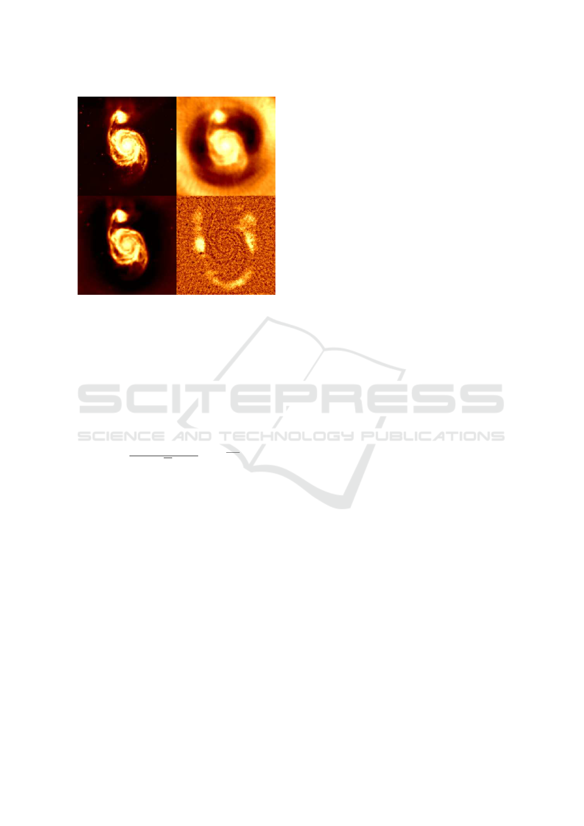
Figure 2: Simulation of observation and reconstruction of

the spiral galaxy M51 using ADMM implemented with PU-

RIFY, including the ground truth (top left), the observed

image (top right), the PURIFY reconstruction (bottom left),

and the residuals (bottom right). We used an ISNR of 30dB,

a pixel size of 0.3

, and an image size of 256 by 256 pixels,

with the sampling pattern for 10 spectral bins as shown in

Figure 1 resulting in 4440 measurements. The structure of

the spiral arms and point sources are recovered well using

PURIFY.

an input signal to noise ratio (ISNR) to determine the

standard deviation of the Gaussian noise, where this

standard deviation is deﬁned as

kΦx

GroundTruth

√

×10

−

ISNR

. (13)

The Fourier sampling pattern of the observation (i.e.

the uv-coverage) is determined by the design of the

SPIDER instrument and the optical spectral coverage.

By combining the entire spectra it is possible to in-

crease the sampling coverage, as explained in Section

2. We use the conﬁguration of Table 1 (shown in Fig-

ure 1).

The results presented in Figure 2 show that an

observation using the proposed SPIDER design can

be effectively reconstructed using PURIFY. Recon-

struction was performed using a Dirac basis and

Daubechies wavelets 1 to 8. While we have used the

design from (Kendrick et al., 2013), where the base-

lines lie on radial spokes, different baseline conﬁgu-

rations may lead to higher quality reconstruction. De-

pending on the structures in the ground truth sky, dif-

ferent baseline conﬁgurations will be more effective

at sampling the sky, leading to more effective recon-

struction of objects and their details. It was recently

shown that the theory of compressive sensing might

lead to more efﬁcient designs (Liu et al., 2018).

In summary, we adapt recent developments in ra-

dio interferometric imaging, leveraging sparsity and

convex optimisation, and show that they are effective

for imaging SPIDER observations. Moreover, recent

developments in efﬁcient uncertainty quantiﬁcation

for radio interferometric imaging can also be adapted

for use with SPIDER (Cai et al., 2018b). The compu-

tational performance of these algorithms can be fur-

ther increased using GPU multi-threading and distri-

bution across nodes of a computing cluster (as imple-

mented in PURIFY already; (Pratley et al., 2019b)).

REFERENCES

Boyd, S. et al. (2011). Distributed optimization and statis-

tical learning via the alternating direction method of

multipliers. Found. Trends Mach. Learn., 3(1):1–122.

Cai, X., Pereyra, M., and McEwen, J. D. (2018a). Uncer-

tainty quantiﬁcation for radio interferometric imaging

- I. Proximal MCMC methods. MNRAS, 480:4154–

4169.

Cai, X., Pereyra, M., and McEwen, J. D. (2018b). Uncer-

tainty quantiﬁcation for radio interferometric imag-

ing: II. MAP estimation. MNRAS, 480:4170–4182.

Duncan, A. et al. (2015). SPIDER: Next Generation

Chip Scale Imaging Sensor. In Advanced Maui Opti-

cal and Space Surveillance Technologies Conference,

page 27.

Fessler, J. A. and Sutton, B. P. (2003). Nonuniform fast

fourier transforms using min-max interpolation. IEEE

Transactions on Signal Processing, 51:560–574.

Jackson, J. I., Meyer, C. H., Nishimura, D. G., and Macov-

ski, A. (1991). Selection of a convolution function

for fourier inversion using gridding [computerised to-

mography application]. IEEE Transactions on Medi-

cal Imaging, 10(3):473–478.

Kendrick, R. et al. (2013). Flat Panel Space Based Space

Surveillance Sensor. In Advanced Maui Optical and

Space Surveillance Technologies Conference, page

E45.

Liu, G., Wen, D., and Song, Z. (2017). Rearranging the

lenslet array of the compact passive interference imag-

ing system with high resolution. In AOPC 2017:

Space Optics and Earth Imaging and Space Naviga-

tion, volume 10463 of Society of Photo-Optical In-

strumentation Engineers (SPIE) Conference Series,

page 1046310.

Liu, G., Wen, D.-S., and Song, Z.-X. (2018). System de-

sign of an optical interferometer based on compressive

sensing. MNRAS, 478:2065–2073.

Onose, A. et al. (2016). Scalable splitting algorithms for

big-data interferometric imaging in the SKA era. MN-

RAS, 462:4314–4335.

Pereyra, M., Bioucas-Dias, J. M., and Figueiredo, M. A. T.

(2015). Maximum-a-posteriori estimation with un-

known regularisation parameters. In 2015 23rd Eu-

PHOTOPTICS 2021 - 9th International Conference on Photonics, Optics and Laser Technology

108

ropean Signal Processing Conference (EUSIPCO),

pages 230–234.

Pratley, L. (2019). Radio Astronomy Image Reconstruc-

tion in the Big Data Era. Doctoral thesis (Ph.D), UCL

(University College London).

Pratley, L., Johnston-Hollitt, M., and McEwen, J. D.

(2019a). A Fast and Exact w-stacking and w-

projection Hybrid Algorithm for Wide-ﬁeld Interfer-

ometric Imaging. ApJ, 874(2):174.

Pratley, L., McEwen, J. D., d’Avezac, M., Cai, X., Perez-

Suarez, D., Christidi, I., and Guichard, R. (2019b).

Distributed and parallel sparse convex optimization

for radio interferometry with PURIFY. arXiv e-prints,

page arXiv:1903.04502.

Pratley, L., McEwen, J. D., et al. (2018). Robust sparse

image reconstruction of radio interferometric obser-

vations with purify. MNRAS, 473:1038–1058.

Ryle, M. and Hewish, A. (1960). The synthesis of large

radio telescopes. MNRAS, 120:220.

Su, T. et al. (2017). Experimental demonstration of inter-

ferometric imaging using photonic integrated circuits.

Opt. Express, 25(11):12653–12665.

Thompson, A., Moran, J., and Swenson, G. (2008). Inter-

ferometry and Synthesis in Radio Astronomy. Wiley.

Yang, J. and Zhang, Y. (2011). Alternating direction algo-

rithms for l1-problems in compressive sensing. SIAM

Journal on Scientiﬁc Computing, 33(1):250–278.

Zernike, F. (1938). The concept of degree of coherence and

its application to optical problems. Physica, 5:785–

795.

Sparse Image Reconstruction for the SPIDER Optical Interferometric Telescope

109