
Robust Anomaly Detection in Time Series through Variational
AutoEncoders and a Local Similarity Score
Pedro Matias
1,2
, Duarte Folgado
1
, Hugo Gamboa
1,3
and Andr
´
e V. Carreiro
1
1
Associac¸
˜
ao Fraunhofer Portugal Research, Rua Alfredo Allen 455/461, Porto, Portugal
2
Faculdade de Ci
ˆ
encias e Tecnologia, FCT, Universidade Nova de Lisboa, 2829-516 Caparica, Portugal
3
Laborat
´
orio de Instrumentac¸
˜
ao, Engenharia Biom
´
edica e F
´
ısica da Radiac¸
˜
ao (LIBPhys-UNL), Departamento de F
´
ısica,
Faculdade de Ci
ˆ
encias e Tecnologia, FCT, Universidade Nova de Lisboa, 2829-516 Caparica, Portugal
Keywords:
Anomaly Detection, Time Series, Variational AutoEncoders, Unsupervised Learning, ECG.
Abstract:
The rise of time series data availability has demanded new techniques for its automated analysis regarding
several tasks, including anomaly detection. However, even though the volume of time series data is rapidly
increasing, the lack of labeled abnormal samples is still an issue, hindering the performance of most supervised
anomaly detection models. In this paper, we present an unsupervised framework comprised of a Variational
Autoencoder coupled with a local similarity score, which learns solely on available normal data to detect
abnormalities in new data. Nonetheless, we propose two techniques to improve the results if at least some
abnormal samples are available. These include a training set cleaning method for removing the influence of
corrupted data on detection performance and the optimization of the detection threshold. Tests were performed
in two datasets: ECG5000 and MIT-BIH Arrhythmia. Regarding the ECG5000 dataset, our framework has
shown to outperform some supervised and unsupervised approaches found in the literature by achieving an
AUC score of 98.79%. In the MIT-BIH dataset, the training set cleaning step removed 60% of the original
training samples and improved the anomaly detection AUC score from 91.70% to 93.30%.
1 INTRODUCTION
In the time-series domain, the ever-increasing data
availability raises the need for automating mining or
analysis processes, within which anomaly detection
is included (Chandola et al., 2009). In essence, this
process refers to the automatic detection of samples
that are not conformant with the overall pattern distri-
bution of a dataset. These samples are anomalies or
outliers, and the process is also known as outlier or
novelty detection (Chandola et al., 2009).
There are three categories of anomaly detection
methods: Statistical, Machine Learning (ML), and
Deep Learning (DL) (Braei and Wagner, 2020). Fo-
cusing on the DL field, conventional supervised ap-
proaches (despite showing quite robust performances)
fail in two main points: their performance is impaired
when classes are not balanced (the classifier learns
well how to classify the majority class and fails at
predicting the remaining classes); and they require
a priori knowledge about abnormalities in the data,
which, in some domains, is challenging (Zhang et al.,
2018). Thus, as normal data is largely more avail-
able than abnormal examples, techniques capable of
detecting abnormal samples without being dependent
on its availability/knowledge are of great interest in
several tasks (Chalapathy and Chawla, 2019).
In this work, we present an unsupervised anomaly
detection framework (with possibility of using la-
beled abnormal samples for performance increasing,
if available) that is exclusively dependent on normal
data to learn. The contributions of this paper essen-
tially rest on the implementation of a VAE (Varia-
tional Autoencoder) that learns the most relevant in-
trinsic structure of normal patterns, the establishment
of a new anomaly score that uses VAEs reconstruc-
tion properties to emphasize local dissimilar regions
relative to the original signals, and the proposal of a
training set cleaning stage that reduces the influence
of possibly corrupted samples on the neural network
performance.
1.1 Background
VAEs are unsupervised deep generative models,
which are able to learn meaningful features of the
Matias, P., Folgado, D., Gamboa, H. and Carreiro, A.
Robust Anomaly Detection in Time Series through Variational AutoEncoders and a Local Similarity Score.
DOI: 10.5220/0010320500910102
In Proceedings of the 14th International Joint Conference on Biomedical Engineer ing Systems and Technologies (BIOSTEC 2021) - Volume 4: BIOSIGNALS, pages 91-102
ISBN: 978-989-758-490-9
Copyright
c
2021 by SCITEPRESS – Science and Technology Publications, Lda. All rights reserved
91

training data and generalize it to a continuous la-
tent distribution (Kingma and Welling, 2019). It uses
Bayesian inference to learn from data and structurally
consists of an encoder, a latent space, and a decoder.
It performs data compression by encoding inputs into
a latent variable distribution, which is randomly sam-
pled and fitted into the decoder, that expands the latent
sampled vector and tries to rebuild the original signal
according to its training distribution knowledge. The
sampling process is not differentiable, a required con-
dition for the backpropagation to train the network.
Thus, a reparametrization trick is introduced, by cre-
ating a stochastic variable from which the latent vec-
tor z can be sampled, using the estimated mean and
standard deviation vectors.
Regarding the loss function, a VAE defines a cus-
tom loss function composed of two different terms: a
reconstruction term, which forces both input and out-
put to be morphologically similar, and a regularizer
term, which approximates each latent variable distri-
bution to a standard normal distribution.
1.2 Related Work
In the past few years, the number of studies fo-
cusing on anomaly detection tasks in time series
data has significantly increased. Most traditional un-
supervised approaches use distance-based methods,
such as nearest-neighbor (Ramaswamy et al., 2000)
or clustering (He et al., 2003) algorithms, to de-
tect anomalies. Density estimation methods (Ma and
Perkins, 2003), by capturing the density distribution
of the training data, and temporal prediction tech-
niques (Pincombe, 2005), taking into account tem-
poral dependency within time series, are other two
different categories. However, these approaches have
higher computational complexity, especially for high-
dimensionality data. Dimensionality reduction tech-
niques may solve the problem, but they will also re-
move detailed information, which can decrease per-
formance (Zhang et al., 2020). More recently, DL-
based anomaly detection models have gained some
popularity in this domain (Chalapathy and Chawla,
2019). Approaches based on generative models like
VAEs and Generative Adversarial Networks (GANs)
have shown quite competitive performances relative
to conventional methods due to their strong gener-
alization, modeling, and reconstruction ability. This
enables the learning of the most relevant structure of
training data, which will be used to build a lower-
dimensional latent space distribution to where sam-
ples can be mapped. The analysis of this latent space
and the samples’ reconstruction quality are common
procedures of several frameworks. Many works de-
veloped techniques based on those two types of deep
generative models for detecting anomalies in time-
series data, such as AnoGan (Schlegl et al., 2017),
MAD-GAN (Li et al., 2019) (which implement GAN
architectures), and VELC (Zhang et al., 2020), Donut
(Xu et al., 2018) (which use VAE models).
2 PROPOSED FRAMEWORK
The proposed framework is composed of a Latent
Representation learning step, based on a VAE model,
an optional training data cleaning process when some
abnormal samples are available and corrupted labels
are expected, and, finally, a new local anomaly score
for the final classification task.
2.1 Latent Space Representation
The first component is a model able to map the in-
put data into a reduced latent space. To this end, a
VAE architecture was implemented. Through a VAE
model trained only with normal samples, the model
is expected to learn a latent space distribution char-
acteristic of normal data, which is pushed to follow a
standard normal distribution. Moreover, for anomaly
detection purposes, the model will be able to success-
fully reconstruct the normal samples, whereas the re-
construction quality of the anomalies is expectedly
worse. Figure 1 presents the implemented architec-
ture.
Latent mean
Latent stddev
Epsilon ~ N(0,1)
Latent Vector (Z)
INPUT
OUTPUT
Sampling
ENCODER DECODER
Conv1D + MaxPooling Conv1D + Upsampling Dense Lambda
Figure 1: Illustration of VAE network, proposed in this ex-
periment.
The proposed architecture contains, essentially,
1D-Convolutional (Conv-1D) and Fully-Connected
(Dense) layers. Each Conv-1D layer is associated
with a pooling/unpooling layer so that data gets com-
pressed and expanded, respectively. Convolution op-
erations are quite useful when feature extraction and
pattern recognition is needed, being, in this case, cru-
cial for either creating a representative normal latent
BIOSIGNALS 2021 - 14th International Conference on Bio-inspired Systems and Signal Processing
92

space and returning suitable reconstructions of nor-
mal samples. Dense layers are used to get the la-
tent vectors and the output signal. The number of la-
tent variables, z
dim
, was set to 10 across experiments,
chosen empirically in preliminary experiments, as
a trade-off between ensuring a robust extraction of
meaningful latent features while avoiding an abrupt
dimensionality reduction by UMAP (Uniform Mani-
fold Approximation and Projection) technique (as it
will be further explained).
Regarding the VAE loss function, for the recon-
struction term, the mean-squared error (MSE) has
been selected to measure the dissimilarity between
original and reconstructed samples. The second
term will calculate the Kullback-Leibler Divergence
(KLD) between each latent variable mean (µ) and
standard deviation (σ), and a standard normal distri-
bution (µ = 0, σ = 1). The final expression is given by
the following equation:
L
VAE
= MSE(X, X
0
)
| {z }
Reconstruction
+β ·
1
2
z
dim
∑
i=1
(µ
2
i
+ σ
2
i
) −1 − log(σ
2
i
)
| {z }
Regularizer
(1)
In equation 1, X and X
0
are the original and re-
constructed signals, respectively, z
dim
is the latent
space dimensionality, and µ and σ are the latent mean
and standard deviation distribution parameters, re-
spectively. A β factor has been included to reduce
the regularization term weight, avoiding a posterior
collapse (Lucas et al., 2019).
2.2 Training Samples Cleaning
A first step to prepare the training is guaranteeing
a good quality annotated dataset. In larger datasets,
where labels have been assigned manually by special-
ists, the probability of wrongfully annotated samples
is higher. Furthermore, a filtering stage is often not
sufficient to improve SNR (signal-to-noise ratio), and
some samples may get considerably distorted, despite
being well labeled. These two issues may hinder the
deep neural network performance. Therefore, in an
attempt to remove corrupted samples from a training
set, a sample selection technique is proposed. We note
that this is applied only to the training set, thus keep-
ing the test and validation sets intact.
Firstly, the approach assumes some anomalies are
known, which are used as a reference to reject normal-
labeled samples to which they are most similar. In
summary, the proposed technique consists of training
the aforementioned VAE model and use its latent rep-
resentation to map the input into a feature space di-
mension, where some samples are rejected based on
their vicinity. The individual steps are explained as
follows:
1. Train the VAE with the Training Set to Clean:
the training set is composed only of normal-
labeled samples. The architecture is the same
used to perform anomaly detection;
2. Extract the Embedding Representation: by ap-
plying the encoder’s compression to the trained
normal and known abnormal samples, the embed-
ded representations become represented by an N-
sized latent vector;
3. Apply UMAP to Extracted Embeddings:
UMAP (McInnes et al., 2020) is a flexible non-
linear dimensionality reduction technique that
finds a lower-dimensional embedding preserving
the most relevant structure of the data. As the
VAE already learns the distribution of normal
data, UMAP is applied to its latent embeddings
and not the raw inputs so that the dimension re-
duction is not too abrupt. Subsequently, the N-
dimensional embeddings are mapped into a two-
dimensional space (given as a parameter);
4. Reject Normal Samples Closer to Abnormal
Ones: first, the minimum Euclidean distance be-
tween each normal sample (from the training set)
and all the abnormal ones is computed. Then,
samples whose minimum distance is above the N
th
percentile of all distances are selected, and the re-
maining rejected. This defines the new, filtered,
training set.
An illustrative scheme summarizing the four steps is
displayed in Figure 2.
We note that as the number of rejected samples
rises, the training set normal variability tends to de-
crease, which can lower the network reconstruction
ability. This trade-off depends on the reject threshold
(N
th
percentile value on step 4), which can be selected
according to each dataset properties, such as the num-
ber of known anomaly types, confidence in the label-
ing process, etc.
2.3 Anomaly Score
A common approach for anomaly detection is based
on comparing a similarity metric between a learned
normality representation vs. outliers, assigning a
score upon which a decision can be made, regarding
if it is an anomalous sample or not. To this end, sev-
eral different scores might be computed. Convention-
ally, the Euclidean distance (L
2
norm) or MSE are the
most common metrics to compare original and recon-
structed signals. However, they provide a global per-
spective, whereas the distortion is often constrained
Robust Anomaly Detection in Time Series through Variational AutoEncoders and a Local Similarity Score
93

ENCODER DECODER
VAE
Normal Samples
S1S2 S3 Sn
...
...
S1S2 S3 Sm
...
...
Abnormal Samples
Latent layer
UMAP representation
Selected sample
Rejected sample
Abnormal sample
...
...
Embeddings
2D-mapping
S1 S2 S3
Sm
...
S1 S2 S3
Sn
...
Figure 2: Illustration of the sample cleaning procedure.
to local segments. Hence, global scores may hide
the correct interpretation of the reconstruction result.
In order to improve this local distortion awareness, a
new local dissimilarity score is proposed. Given X
and X
0
, the original and reconstructed samples, re-
spectively, and d, the point-to-point Euclidean dis-
tance vector between both, the highest dissimilar sam-
ples are selected through the condition:
D
M
= {d
i
, i f d
i
> P
M
}
0 <i< |d|
(2)
In equation 2, d
i
∈ d, P
M
is the M
th
percentile of
d vector, and D
M
is the vector containing the M%
highest-scored points. The final anomaly score is the
average over the defined points:
S
local
=
1
|D
M
|
|D
M
|
∑
i=1
D
i
(3)
This score is expected to improve the detection of lo-
cal anomalies, of special interest in signals with sub-
patterns such as the ECG (electrocardiogram). Figure
3 illustrates the idea behind this new score.
Normal Reconstruction Abnormal Reconstruction
S
local
E
dist
S
local
> E
dist
Original
Reconstructed
% highest-scored points
Figure 3: Visual representation of the proposed local
anomaly score. S
local
and E
dist
refer to the local score and
global Euclidean distance, respectively.
2.4 Evaluation
The evaluation stage allows to objectively assess the
performance of a given model and infer about its be-
havior under different conditions. In this work, eval-
uation is based on Receiver Operating Characteristic
(ROC) curve, its Area under the Curve (AUC), and
for a given threshold, the (Balanced) Accuracy and
F1-score.
Furthermore, an optimal threshold value can be
computed, corresponding to the best separation be-
tween Normal and Abnormal distributions. For this,
we calculate Youden’s J score (Ruopp et al., 2008),
and find where its maximum occurs:
J = T PR − FPR (4)
In equation 4, TPR and FPR designates the True Pos-
itive Rate and False Positive Rate, correspondingly.
Note that this threshold value should be computed
for the validation set (as it depends on known abnor-
mal samples), since the testing set should not be re-
flected in any model decision. However, for compar-
ison purposes with other works who choose the op-
timal threshold based on the testing set, we include
this in our analysis. The general procedure of train-
ing, validation and test stages is summarized and il-
lustrated by Figure 4.
VAE
Training
Threshold
choice
Hypermarameter tuning
Training
Set
Testing
Set
Training
Split
Validation
Split
Dataset
Pre-processing
ROC curve
ROC curve
Evaluation
metrics
Figure 4: Overall training procedure scheme.
BIOSIGNALS 2021 - 14th International Conference on Bio-inspired Systems and Signal Processing
94
3 APPLICATIONS
The proposed framework was validated in two
use-cases, both concerning the ECG domain: the
ECG5000 dataset and the MIT-BIH Arrhythmia
dataset.
3.1 ECG5000 Dataset
The ECG5000 dataset is an ECG database released by
Eamonn Keogh and Yanping Chen, and publicly avail-
able in the UCR Time Series Classification archive
(Dau et al., 2019). It contains 5000 heartbeats (ex-
tracted from a single patient) with a length of 140
points each. 4500 heartbeats (80%) were held for test-
ing and 500 for training tasks (20%), as shown in Ta-
ble 1.
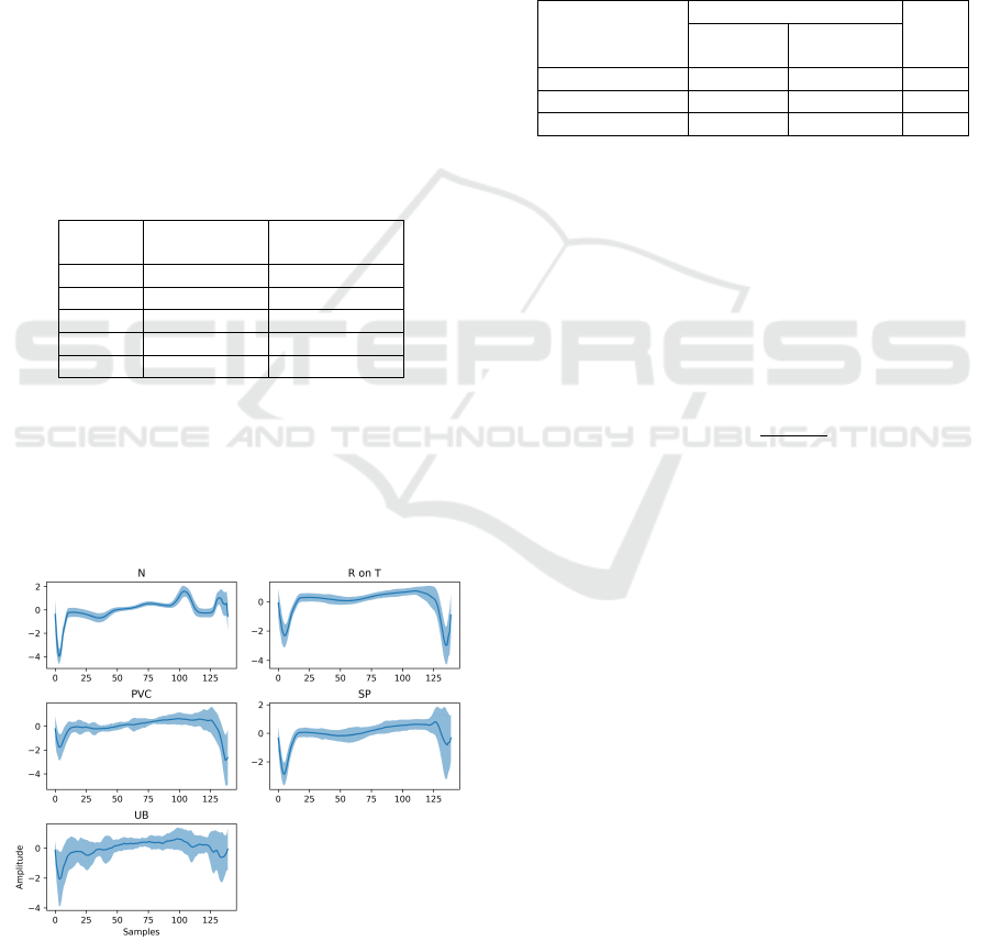
Table 1: Overview of samples distribution over classes N
(Normal), R-on-T (R-on-T Premature Ventricular Contrac-
tion), PVC (Premature Ventricular Contraction), SP (Supra-
ventricular Premature beat), and UB (Unclassified Beat).
Class Train Test
N 292 (58.4%) 2627 (58.4%)
R-on-T 177 (35.4%) 1590 (35.4%)
PVC 10 (2.00%) 86 (1.92%)
SP 19 (3.80%) 175 (3.88%)
UB 2 (0.40%) 22 (0.48%)
The majority class (N) was considered the Normal
class, while the remaining classes were grouped into
a single Abnormal class.
The morphological variability of each class is
shown in Figure 5.
Figure 5: Classes morphological variability on ECG5000
dataset. The highlighted regions indicate the overall aver-
age amplitude (dark blue line) surrounded by one standard
deviation, in both sides (light blue).
3.1.1 Dataset Splitting
For validation purposes, the original training set has
been divided into two subsets: one for training the
model (X
train
) and the other for hyperparameter tuning
(X
val
), as done in (Pereira and Silveira, 2019), with a
splitting ratio (train/validation) of 80/20, respectively.
For testing purposes, a different set (X
test
) was already
predefined. Table 2 summarizes the dataset splitting
procedure.
Table 2: Overview of each set number of samples, on
ECG5000 dataset.
Class
Train
Test
Training
(80%)
Validation
(20%)
Normal class 234 58 2697
Abnormal class - 208 1803
Total 234 266 4500
3.1.2 Pre-processing
As a preprocessing step, we applied a single normal-
ization process to the input signals to keep the com-
parison with other techniques as fair as possible.
• Normalization: dividing each signal by the max-
imum of its absolute ensures the data has an am-
plitude range between -1 and 1.
X
0
=
X
max |X|
(5)
X and X
0
refer to the original and pre-processed
signals, respectively.
3.1.3 Training Stage
This step regards the actual training of the model,
and hyperparameter optimization, to achieve the high-
est possible reconstruction difference between normal
and abnormal validation samples. If abnormal data is
not available (purely unsupervised setting), this step
tries to avoid the network’s overfitting. Table 3 indi-
cates the best settings adopted for this dataset.
3.2 MIT-BIH Arrhythmia Database
The MIT-BIH Arrhythmia Database is a clinical
database (Moody and Mark, 2001), where records are
ECG signals collected from 47 subjects for two differ-
ent leads/channels. There were extracted 48 half-hour
excerpts from 4000 randomly chosen 24-hour ambu-
latory records. For this analysis, lead MLII was cho-
sen since it is present in most records.
Robust Anomaly Detection in Time Series through Variational AutoEncoders and a Local Similarity Score
95
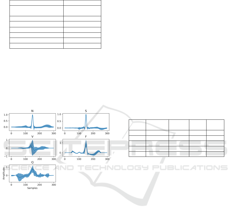
Table 3: Overview of VAE model training hyperparameters,
applied to ECG5000 dataset analysis.
Parameters 49012
Loss function
MSE + β · D
KL
[β = 0.01]
Optimizer Adam
Learning-Rate 1 × 10
−3
Epochs 100
Early Stopping patience 6 epochs
Activation functions TanH and Linear
Batch size 16
Following AAMI (Association for the Advance-
ment of Medical Instrumentation) recommendations
(da S. Luz et al., 2016), the selected heartbeats are
labeled into five different classes: N (Normal), and
anomalies S (Supraventricular ectopic), V (Ventricu-
lar ectopic), F (Fusion beat), Q (unknown beat). The
overall shape of each heartbeat class is presented in
Figure 6.
Figure 6: Classes’ morphological variability on MIT-BIH
Arrhythmia dataset. The highlighted regions indicate the
overall average amplitude (dark blue line) surrounded by
one standard deviation, in both sides (light blue).
From Figure 6, anomalies from classes S and F
seem the most challenging to detect since their mor-
phology is similar to that of the N class, with smaller
local deviations rather than global deviations, as for
the V and Q classes.
3.2.1 Dataset Splitting
Following the method proposed by Chazal et al.
(Philip de Chazal et al., 2004), the dataset was divided
into DS1 and DS2 subsets, each one containing ECG
records of 22 different individuals. Additionally, DS1
was further split to create a validation set in order to
guide the training stage in terms of hyperparameter
tuning.
Since the goal of this experiment focuses on de-
tecting morphological anomalies (and not temporal
ones, since single heartbeats are evaluated instead of
longer windows), AAMI recommended classes were
partially changed. This way, in opposition to what
AAMI recommends:
• L, R, j, and e (left and right bundle branch block,
nodal and atrial escape beats, respectively) labels
were removed from class N since bundle branch
blocks and escape beats are both a type of arrhyth-
mia. Thus, only N-labeled beats defined the Nor-
mal class;
• Patient number 108 has been removed from the
training set since its Normal-labeled cardiac cy-
cles are morphologically distinct from those char-
acteristic of a lead II acquisition.
Table 4 displays the labels assigned to each class
(da S. Luz et al., 2016), as well as the number of sam-
ples associated.
Table 4: Overview of each set samples distribution over all
classes on MIT-BIH Arrhythmia dataset.
Class Labels
DS1
(Train)
DS1
(Val.)
DS2
(Test)
N N 31149 5149 36380
S a, A, J, S - 939 1834
V V, E - 3768 3216
F F - 412 388
Q /, f, Q - 8 7
Training and Validation (DS1): 101, 106, 109, 112,
114, 115, 116, 118, 119, 122, 124, 201, 203, 205, 207,
208, 209, 215, 220, 223, 230.
Testing (DS2): 100, 103, 105, 111, 113, 117, 121,
123, 200, 202, 210, 212, 213, 214, 219, 221, 222, 228,
231, 232, 233, 234. For anomaly detection purposes,
class N defined the Normal class, and the remaining
(S, V, F, Q) the Abnormal class.
We note that DS1 was split by individual so that
the training and validation sets did not share heart-
beats of the same patient. Therefore, approximately
19% of the individuals present in DS1 (4 out of 21)
constituted the validation set and the remaining 17 the
training set.
3.2.2 Pre-processing
Signal pre-processing is a crucial step, especially re-
garding physiological signals as the ECG, consider-
ing all possible noise sources that could hinder any
subsequent model performance. The following pre-
processing steps were applied:
1. Butterworth Bandpass Filter: a fifth-order fil-
ter, with lower and higher cutoff frequency at 0.5
and 30 Hz, respectively. It stabilizes the baseline
BIOSIGNALS 2021 - 14th International Conference on Bio-inspired Systems and Signal Processing
96
drift and attenuates high-frequency noise compo-
nents.
2. Median Filter: with a kernel size of 0.6 seconds
(average heartbeat duration), it is similar to a mov-
ing average filter, except the median is used in-
stead of the mean. It helps to improve baseline
correction and remove some artifacts (Lee et al.,
2020).
3. Heartbeat Extraction: it consists of selecting a
neighborhood surrounding each R-peak annota-
tion. This interval is calculated based on the cur-
rent heart-rate (BPM) and is defined as half the
associated period, in both directions.
Beat
edges
=
R
idx
± 0.5 ·
60· f s
BPM
if BPM > 70
R
idx
± 0.5 ·
60· f s
70
if BPM ≤ 70
(6)
The extracted cycles usually differ in length, so, in a
last pre-processing step, all heartbeats were padded
with zeros on both sides so that they can fit the VAE
architecture, as well as normalized following equation
5. Note the zeros added from padding are not consid-
ered for anomaly scores calculation.
3.2.3 Training Stage
As done for the ECG5000 dataset, the best possi-
ble hyperparameter settings obtained for MIT-BIH Ar-
rhythmia are the same as those presented in Table
3, except the Parameters (60372) and the Batch size
(32).
4 RESULTS AND DISCUSSION
4.1 ECG5000 Dataset
Considering the low number of training samples on
this dataset, the sample cleaning step was not applied
since it would further reduce the number of normal
samples available to train the VAE network.
4.1.1 Signal Reconstruction
The reconstruction ability of this network dictates
its anomaly detection performance. Figures 7 and 8
present some visual examples comparing an original
signal to its corresponding reconstruction, accompa-
nied by the computed local anomaly score.
As shown in Figure 7, normal samples have their
intrinsic variability but their general morphological
structures remain visible, whatever the level of noise
Figure 7: Normal samples reconstruction on ECG5000
dataset. Input and reconstructed samples are plotted in blue
and orange colors, respectively, and most dissimilar points
are highlighted in red. Computed anomaly scores are de-
fined above each subfigure.
and shape distortion. These are the main features the
VAE is supposed to learn during training. Although
reconstruction is not perfect, it is still much closer
than for anomalous heartbeats (Figure 8), a require-
ment for anomaly detection.
Figure 8: Abnormal samples reconstruction on ECG5000
dataset. Input and reconstructed samples are plotted in blue
and orange colors, respectively, and most dissimilar points
are highlighted in red. Computed anomaly scores are de-
fined above each subfigure.
Regarding the examples presented in Figure 8, the
VAE encoder maps each one of these abnormal sam-
ples to a continuous latent space of normal heartbeats.
As it can be noticed, even though some abnormal
samples are generally similar to its normal reconstruc-
tion, local dissimilarities can make them distinguish-
able.
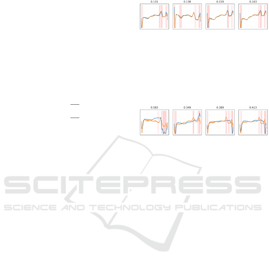
4.1.2 Anomaly Detection
The results of anomaly detection are evaluated
through the computation of AUC, Accuracy, and F1-
score associated with each ROC curve and chosen
threshold. First, the reconstructed scores (calculated
on validation set samples) are used to compute a ROC
curve and calculate an optimal threshold that allows
the ideal separation between normal and abnormal re-
construction scores (Figure 9). The separation be-
tween normal and abnormal distributions is clear, be-
ing quantitatively confirmed by a high AUC score of
99.60%. The optimal threshold of 0.267 was found
through Youden’s J score.
Evaluating the testing set, as seen in Figure 10,
normal and abnormal reconstruction score distribu-
tions seem quite well separated, which implies the
VAE model has learned meaningful features charac-
teristic of normal patterns. While the model can re-
construct normal heartbeats reliably, most abnormal
heartbeats cannot be retrieved successfully. The ROC
curve shape and the AUC score of 98.70%, displayed
Robust Anomaly Detection in Time Series through Variational AutoEncoders and a Local Similarity Score
97
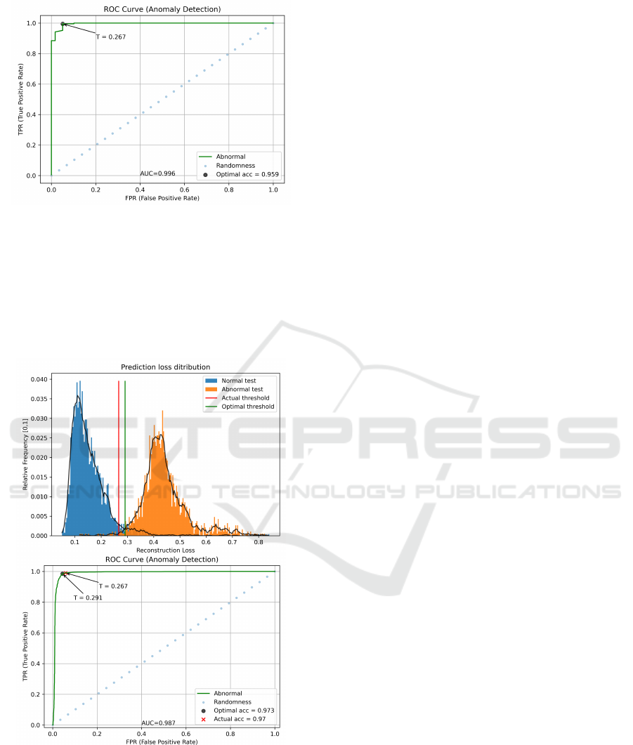
Figure 9: Representation of the ROC curve computed con-
sidering Normal and Abnormal anomaly score distributions,
applied to the validation set on ECG5000 dataset. The
threshold value is marked with a ’T ’ character.
in Figure 10, confirm this visual inference. Further-
more, the selected threshold also generalizes well in
this set, showing an accuracy of 97.00% , quite simi-
lar to the optimal threshold value for the test set.
Figure 10: Representation of anomaly scores distribution
(top) and the corresponding ROC curve (bottom), applied
to the testing set on ECG5000 dataset. Selected and Opti-
mal threshold values are marked with a ’T ’ character in the
bottom image.
4.1.3 Evaluation Metrics
As the ECG5000 dataset has already been employed
in previous works, comparing our approach to other
supervised and unsupervised techniques is important
to better discuss its advantages and limitations, as
well as positioning it within the anomaly detection
field. Table 5 presents the results of some super-
vised and unsupervised techniques using the same
dataset. Although supervised approaches generally
solve a multi-class classification problem, the class
imbalance makes most samples belonging to Normal
and R-on-T PVC classes, so the approximation to a
two-class problem (anomaly detection) will not cause
much interference on the evaluation scores. Optimal
and Selected rows of our proposal (Ours) refers to
the scores obtained through optimal and (validation)
selected thresholds, respectively. The Selected ver-
sion uses the threshold chosen based on the valida-
tion set (requires known anomalies and is thus semi-
supervised at this level), and it is a more reasonable
choice since it does not require knowing labels of the
testing set. The Optimal approach, which considers
the labels in the testing set, was only used for com-
parison purposes with the methods from (Pereira and
Silveira, 2019).
The dataset split employed in (Pereira and Sil-
veira, 2019) is unknown. Thus, for a fair compari-
son, we avoided a single dataset splitting evaluation,
running our model ten times (ten different splits), and
averaging the results over these runs. For comparison,
VRAE (Pereira and Silveira, 2019), SPIRAL-XGB
(Lei et al., 2017), F-t ALSTM-FCN (Karim et al.,
2018), SAE-C (Malhotra et al., 2017), and oFCMdd
(Liu et al., 2018) approaches were included in Table
5. In this table, S/U column cells usually contain two
characters to distinguish the supervision level of both
learning stage (first character) and threshold choice
(second one). One single character indicates the same
supervision level in both aspects. Moreover, super-
vised and unsupervised best scores are underlined and
bolded, correspondingly.
The comparison with the VRAE models will
be emphasized since they are also based on VAEs.
The three presented VRAE techniques focus on us-
ing a post-processing technique to analyze the VAE’s
latent representation, while the model proposed in
this work uses a post-processing similarity score be-
tween input and reconstructed signals. In terms of the
AUC score, the model proposed in this work (Ours)
achieved the highest one, meaning it can achieve the
best separation between normal and abnormal sample
distributions. Regarding Accuracy and F1-score, the
VRAE+SVM approach ends up reaching the highest
scores. Nevertheless, amongst unsupervised methods,
BIOSIGNALS 2021 - 14th International Conference on Bio-inspired Systems and Signal Processing
98
our proposed model has still obtained the highest Ac-
curacy and F1 scores. Concerning the Selected alter-
native of the proposed framework, as expected, scores
have decreased, since the testing set labels are used
exclusively for evaluation and not for optimal thresh-
old choices, but we note that this is what can be an-
ticipated for new, real-world data samples. Summing
up, comparing the training settings of both proposed
and VRAE approaches, the former was trained with
57 training epochs and 49 012 trainable parameters
against 1500 epochs and 273 420 trainable parameters
from the latter, which suggests a higher computational
efficiency. Thus, as the proposed model is structurally
simpler and achieves similar or better results, it can be
a more reasonable choice, especially if at least some
anomalous samples are available.
4.2 MIT-BIH Arrhythmia Database
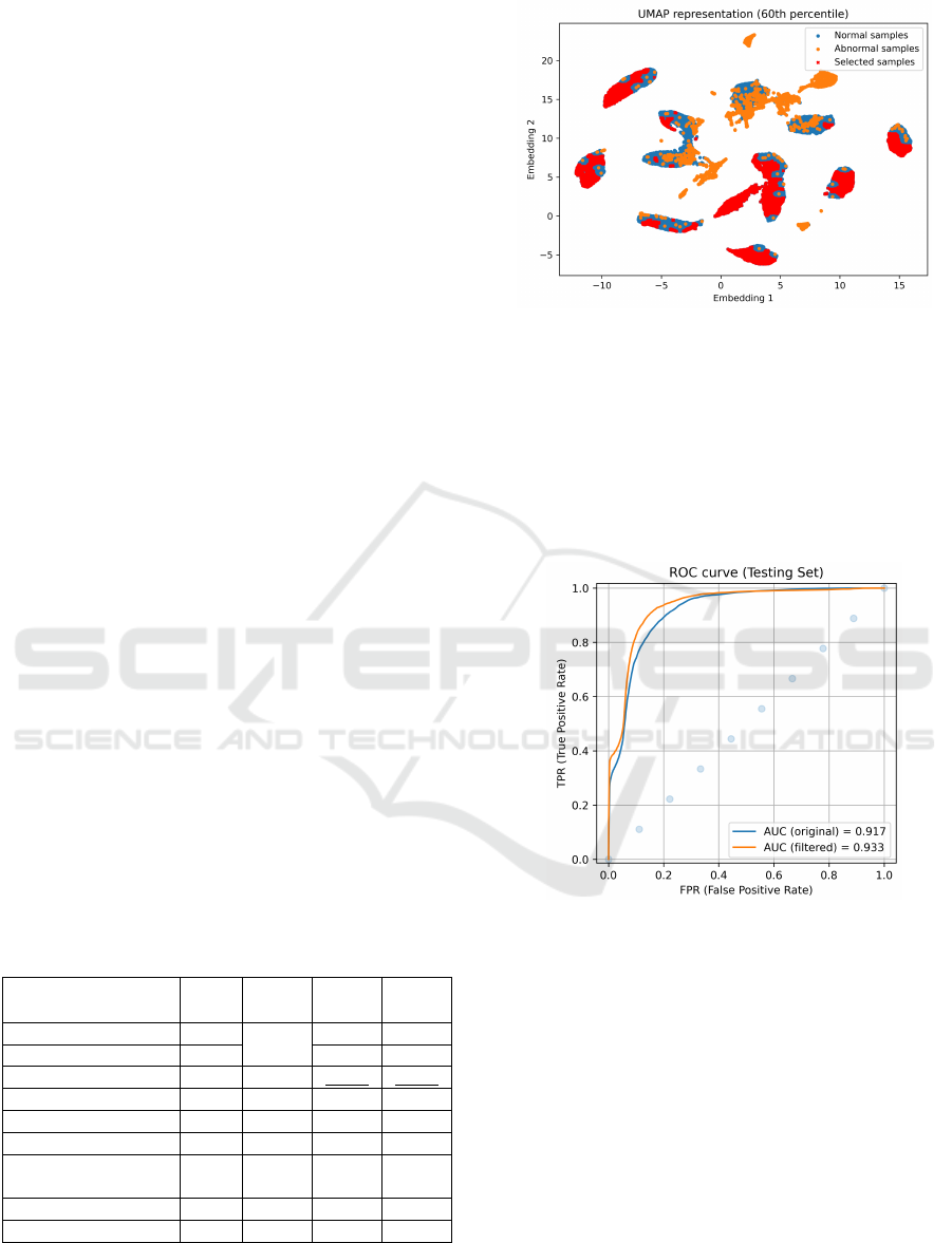
4.2.1 Sample Cleaning
Before training the network for anomaly detection,
training set cleaning was performed. As explained
before, normal and abnormal embedding vectors were
extracted by the originally trained VAE encoder and
mapped into a 2D-plan using the UMAP algorithm.
Finally, a set of [20, 40, 60, 80] percentiles was eval-
uated to assess the influence of the level of sam-
ple rejection on the reconstruction ability, measured
in terms of AUC scores. The 60th percentile level
(where 40% of the training samples were selected)
returned the best score. The 2D map and the corre-
sponding sample selection are shown in Figure 11.
The number of training normal samples has thus
been reduced from 31 149 to 12 460 (60% samples
removed). Comparing the ROC curves of anomaly
score distributions, the filtered training achieved an
Table 5: Overview of models performances on the
ECG5000 dataset.
Model S/U
a
AUC
(%)
Acc
b
(%)
F1
c
(%)
Ours (selected) U+S
98.79
96.86 95.75
Ours (optimal) U+S 97.11 96.01
VRAE + SVM S+S 98.36 98.43 98.44
VRAE+Wasserstein U+S 98.19 95.10 94.61
VRAE + k-Means U 95.91 95.96 95.22
SPIRAL-XGB S 91.00 - -
F-t
ALSTM-FCN
S - 94.96 -
SAE-C S - 93.40 -
oFCMdd U - - 80.84
a
Supervised/Unsupervised
b
Accuracy
c
F1-score
Figure 11: UMAP two-dimensional projection of samples’
latent vectors. The best score was achieved by rejecting
60% of the normal samples closest to the known abnormal
ones.
AUC of 95.90% against 95.80% from the original one
(on the validation set), and 93.30% against 91.70%,
respectively (on testing set). Figure 12 presents the
same testing ROC curves before and after applying
the sample cleaning process.
Figure 12: ROC curves built through inference on the test-
ing set. Blue and orange curves correspond to networks
with and without training set cleaning, respectively.
For both sets, the cleaning stage has been shown
to improve the network performance regarding the
anomaly detection task. Both AUC scores overcame
the original ones, meaning there were some heartbeats
in the original training hindering the model perfor-
mance, either by wrongful annotations, or significant
distortions.
4.2.2 Signal Reconstruction
In Figures 14 and 13 some examples of normal and
abnormal heartbeats, respectively, are displayed, to-
gether with their corresponding reconstructions and
anomaly scores.
Robust Anomaly Detection in Time Series through Variational AutoEncoders and a Local Similarity Score
99
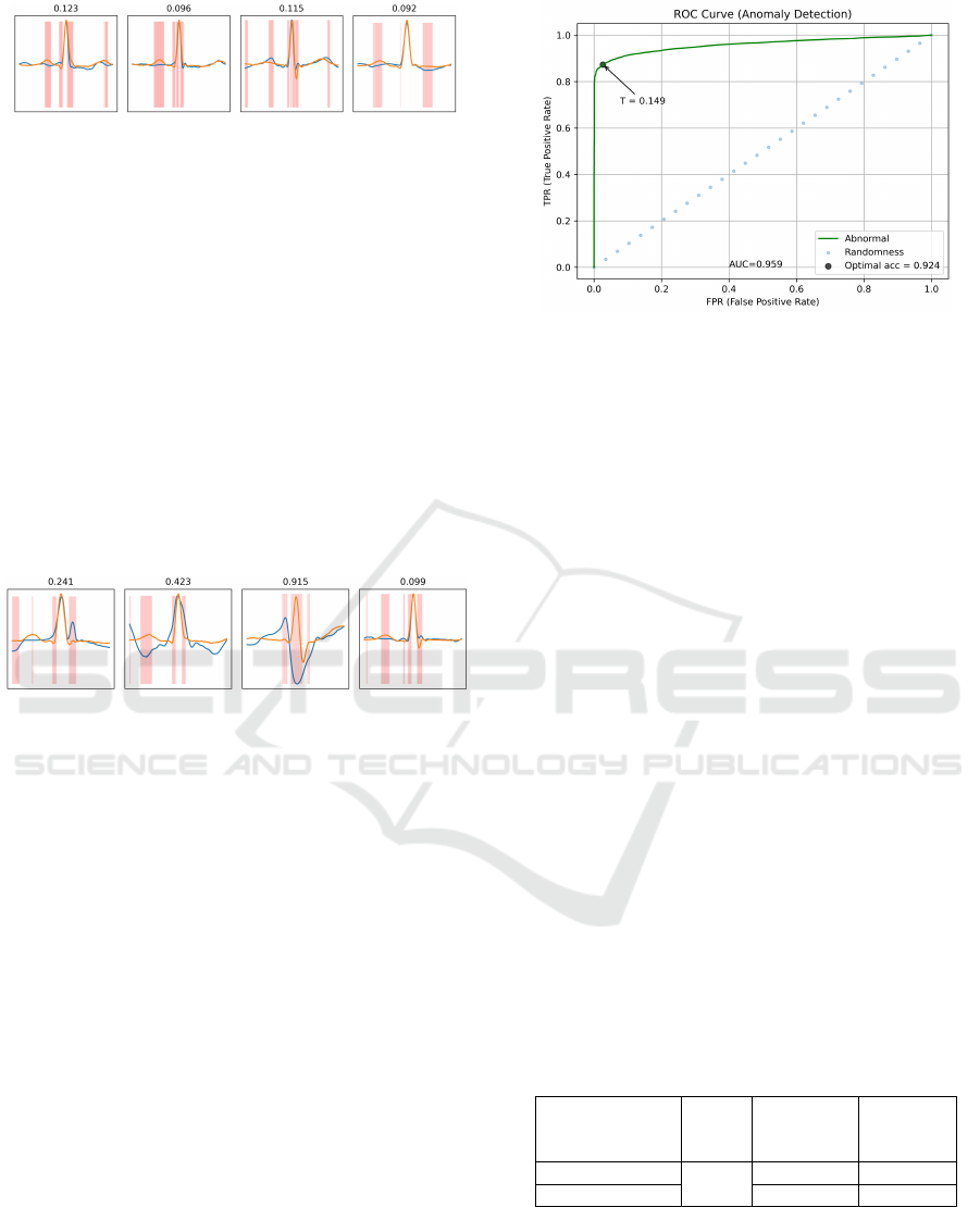
Figure 13: Normal ECG heartbeats reconstruction on MIT-
BIH dataset. Original and reconstructed signals are set with
a blue and an orange line, respectively, and the most dissim-
ilar points are highlighted in red. Reconstruction scores are
above each subfigure.
Regarding normal heartbeats, they seem to be
quite well reconstructed by the network (Figure 13).
It is clear that the model has learned the general mor-
phological behavior of a normal cardiac cycle pat-
tern on lead II. There are some heartbeats revealing a
certain level of variability (like high-frequency noise,
any shorter/larger complex) which were not present
in the training samples. Nonetheless, in the majority
of cases, the network can deal with it, adapting the
output to the input as much as the normal latent space
allows, and looking always towards minimizing the
reconstruction loss.
Figure 14: Abnormal ECG heartbeats reconstruction on
MIT-BIH dataset. Original and reconstructed signals are
set with a blue and an orange line, respectively, and the
most dissimilar points are highlighted in red. Reconstruc-
tion scores are above each subfigure.
Abnormal samples are mapped onto a normal
heartbeat latent space, so the network tries to recon-
struct the input using only normal characteristics of
the cardiac cycle. As expected, the reconstruction
quality is worse in this case, which translates into
higher anomaly scores (Figure 14).
4.2.3 Anomaly Detection
After training the model, thresholds must be defined
and metrics computed on validation and test sets, con-
cerning the evaluation of the anomaly detection per-
formance.
Firstly, anomaly scores (computed between origi-
nal and reconstructed samples) are calculated for the
validation set, and the threshold which better sepa-
rates normal and abnormal score distributions (Fig-
ure 15) is chosen. This value is then used to evaluate
the test set (Figure 16). Analyzing the ROC curve
in Figure 15 and corresponding AUC score (95.90%),
they suggest normal and abnormal score distributions
in the validation set are well separated.
Figure 15: Representation of the ROC curve computed con-
sidering validation set samples, on MIT-BIH dataset. The
threshold value is marked with a ’T ’ character.
Observing the anomaly score distributions in Fig-
ure 16, the fact the testing set has a much higher vol-
ume of data also implies the presence of more normal
corrupted samples, resulting in a distribution curve
with a long tail. Regarding the abnormal distribu-
tion, the presence of a greater number of examples
from class S in the testing set (Table 4), whose mor-
phology is quite similar to class N samples (Figure
6), causes some overlap between both distributions.
Nevertheless, the degree of superposition is not suffi-
ciently high to impair the model’s performance, still
achieving an AUC score of 93.32%.
4.2.4 Evaluation Metrics
In order to make the previous inferences quantifi-
able, Table 6 summarizes the metrics used to evaluate
the testing set, considering both optimal and selected
thresholds as the separation boundary between nor-
mal and abnormal samples. We present the optimal
threshold results to assess how dependent the model
is on this parameter. Due to an extreme imbalance be-
tween the size of Normal and Abnormal classes, bal-
anced scores seemed to be the most suitable for this
analysis: Balanced Accuracy and averaged F1-score.
Table 6: Overview of models performances on MIT-BIH
Arrhythmia dataset.
Model
AUC
(%)
Balanced
Accuracy
(%)
F1-score
(%)
Ours (selected)
93.32
87.71 75.67
Ours (optimal) 87.77 76.55
In absolute terms, these results are worse than
the ones obtained for the ECG5000 dataset. In
this case, the higher variability level of the MIT-
BIH Arrhythmia dataset hinders the reconstruction of
some N-labeled samples possessing an unusual shape.
Nonetheless, the earlier cleaning step has helped to
BIOSIGNALS 2021 - 14th International Conference on Bio-inspired Systems and Signal Processing
100
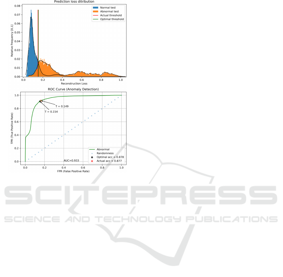
Figure 16: Representation of anomaly scores distribution
(top) and the corresponding ROC curve (bottom), applied
to the testing set on MIT-BIH Arrhythmia dataset. Selected
and Optimal threshold values are marked with a ’T ’ charac-
ter in the bottom image.
obtain slightly better performance with much less
training examples, which must be highlighted.
Using the same overall dataset, according with
(Llamedo and Mart
´
ınez, 2011), Chazal et al. and
Llamedo et al. proposed two different heartbeat clas-
sifiers following the same AAMI five classes and
dataset splitting, having reached averaged F1-scores
of 77.80% and 68.78%, respectively, against 75.67%
from the model proposed in this work. It must be
stressed such a comparison should be made carefully,
since, on one hand, the proposed model is unsuper-
vised in the sense it does not learn from any abnormal
sample, unlike the other two classifiers (supervised).
On the other hand, this work has removed L, R, j, and
e labels from the Normal (N) class, which was not
performed by the other authors.
5 CONCLUSIONS
In this paper, an unsupervised anomaly detection
framework (only dependent of Normal data at the
training level) is proposed for time series analysis.
It was introduced to overcome two main issues: the
strict dependence that supervised models have on ab-
normal data availability, as well as the necessity to
improve the detection of anomalies whose abnormal-
ity regions are local rather than global (being possibly
masked behind global similarity scores). The frame-
work explored the reconstruction ability of VAEs cou-
pled with a local similarity score. Additionally, a
sample cleaning step was included to alleviate the
weight of distorted or wrongly annotated training
samples in the model performance.
The framework was evaluated using two different
ECG datasets: ECG5000 and MIT-BIH Arrhythmia.
In ECG5000 dataset, the goal rested on distinguish-
ing between N-labeled (Normal) heartbeats and re-
maining abnormalities by computing the local simi-
larity score between original and reconstructed sam-
ples. Normal and Abnormal score distributions were
well separated, showing high AUC (98.79%), accu-
racy (97.11%) and F1-score (96.01%), overcoming
other recent unsupervised approaches and showing
competitive results relative to the supervised ones. In
addition, the proposed architecture is structurally sim-
pler and computationally cheaper than the other ap-
proaches, turning it into a more reasonable choice for
anomaly detection.
Regarding the MIT-BIH Arrhythmia dataset, the
analysis focused on separating N-labeled (Normal)
samples from four other types of abnormal heartbeats,
grouped in one single Abnormal class. Here, the sam-
ple cleaning step was applied, and improved the net-
work ability to reasonably reconstruct Normal sam-
ples and even worse Abnormal ones, as desired. For
the test set, the filtered training (40% of the original
samples) increased the AUC score from 91.70% to
93.30%. Balanced accuracy and averaged F1-score
metrics reached 87.77% and 76.55%, respectively.
We found that this testing set has a greater heartbeat
variability, and the dataset contains more challenging
anomaly types (e.g. S and F classes). Nevertheless,
the results are still promising.
As future work, further analysis could con-
sider the local reconstruction score exploring not
only amplitude-related distances but also temporally-
related ones. This could help distinguish other types
of anomalies such as specific arrhythmia types typi-
cally affecting the P wave or the QRS complex, for
instance. Moreover, instead of a predefined score,
a posterior model (e.g. a neural network) might be
trained to measure, more precisely, the degree of mor-
phological dissimilarity between reconstructed and
original signals. In this context, one could also in-
clude a loss term in the VAE to explore the locality of
patterns, learning different weights for different cycle
segments. A different approach might explore a fu-
sion between reconstruction error (as proposed here)
Robust Anomaly Detection in Time Series through Variational AutoEncoders and a Local Similarity Score
101

and latent space analysis (as done for VRAE) for com-
plementary gains in performance. Finally, an even-
tual detection of out-of-domain patterns (e.g. unde-
sired signals corruption, noise, artifacts) could be per-
formed making the VAE learn both normal and ab-
normal domain-patterns, keeping the class of interest
(anomaly) on those kinds of oscillations.
ACKNOWLEDGEMENTS
The project OPERATOR - Digital Transformation in
Industry with a Focus on the Operator 4.0 (OPERA-
TOR - NORTE-01-0247-FEDER-045910) leading to
this work is co-financed by the ERDF - European Re-
gional Development Fund through the North Portugal
Regional Operational Program and Lisbon Regional
Operational Program and by the Portuguese Foun-
dation for Science and Technology - FCT under the
MIT Portugal Program (2019 Open Call for Flagship
projects - Digital Transformation in Industry).
REFERENCES
Braei, M. and Wagner, S. (2020). Anomaly detection in
univariate time-series: A survey on the state-of-the-
art.
Chalapathy, R. and Chawla, S. (2019). Deep learning for
anomaly detection: A survey.
Chandola, V., Banerjee, A., and Kumar, V. (2009).
Anomaly detection: A survey. ACM Comput. Surv.,
41(3).
da S. Luz, E. J., Schwartz, W. R., C
´
amara-Ch
´
avez, G., and
Menotti, D. (2016). ECG-based heartbeat classifica-
tion for arrhythmia detection: A survey. Computer
Methods and Programs in Biomedicine, 127:144 –
164.
Dau, H. A., Bagnall, A., Kamgar, K., Yeh, C.-C. M., Zhu,
Y., Gharghabi, S., Ratanamahatana, C. A., and Keogh,
E. (2019). The ucr time series archive.
He, Z., Xu, X., and Deng, S. (2003). Discovering cluster-
based local outliers. Pattern Recognition Letters,
24(9):1641 – 1650.
Karim, F., Majumdar, S., Darabi, H., and Chen, S. (2018).
LSTM fully convolutional networks for time series
classification. IEEE Access, 6:1662–1669.
Kingma, D. P. and Welling, M. (2019). An introduction to
variational autoencoders. Foundations and Trends
R
in Machine Learning, 12(4):307–392.
Lee, M., Song, T.-G., and Lee, J.-H. (2020). Heart-
beat classification using local transform pattern fea-
ture and hybrid neural fuzzy-logic system based on
self-organizing map. Biomedical Signal Processing
and Control, 57:101690.
Lei, Q., Yi, J., Vaculin, R., Wu, L., and Dhillon, I. S. (2017).
Similarity preserving representation learning for time
series analysis. CoRR, abs/1702.03584.
Li, D., Chen, D., Shi, L., Jin, B., Goh, J., and Ng, S.-K.
(2019). MAD-GAN: Multivariate anomaly detection
for time series data with generative adversarial net-
works.
Liu, Y., Chen, J., Wu, S., Liu, Z., and Chao, H. (2018).
Incremental fuzzy C medoids clustering of time se-
ries data using dynamic time warping distance. PLOS
ONE, 13(5):1–25.
Llamedo, M. and Mart
´
ınez, J. P. (2011). Heartbeat classifi-
cation using feature selection driven by database gen-
eralization criteria. IEEE transactions on bio-medical
engineering, 58:616–25.
Lucas, J., Tucker, G., Grosse, R., and Norouzi, M. (2019).
Don’t blame the ELBO! a linear VAE perspective on
posterior collapse.
Ma, J. and Perkins, S. (2003). Time-series novelty detection
using one-class support vector machines. volume 3,
pages 1741 – 1745 vol.3.
Malhotra, P., TV, V., Vig, L., Agarwal, P., and Shroff, G.
(2017). TimeNet: Pre-trained deep recurrent neural
network for time series classification.
McInnes, L., Healy, J., and Melville, J. (2020). UMAP:
Uniform manifold approximation and projection for
dimension reduction.
Moody, G. and Mark, R. (2001). The impact of the
MIT-BIH arrhythmia database. IEEE engineering in
medicine and biology magazine : the quarterly mag-
azine of the Engineering in Medicine & Biology Soci-
ety, 20:45–50.
Pereira, J. and Silveira, M. (2019). Unsupervised repre-
sentation learning and anomaly detection in ECG se-
quences. International Journal of Data Mining and
Bioinformatics, 22:389–407.
Philip de Chazal, O’Dwyer, M., and Reilly, R. B.
(2004). Automatic classification of heartbeats us-
ing ECG morphology and heartbeat interval fea-
tures. IEEE Transactions on Biomedical Engineering,
51(7):1196–1206.
Pincombe, B. (2005). Anomaly detection in time series of
graphs using ARMA processes. ASOR Bull, 24.
Ramaswamy, S., Rastogi, R., and Shim, K. (2000). Effi-
cient algorithms for mining outliers from large data
sets. volume 29, pages 427–438.
Ruopp, M., Perkins, N., Whitcomb, B., and Schisterman, E.
(2008). Youden index and optimal cut-point estimated
from observations affected by a lower limit of detec-
tion. Biometrical journal. Biometrische Zeitschrift,
50:419–30.
Schlegl, T., Seeb
¨
ock, P., Waldstein, S. M., Schmidt-Erfurth,
U., and Langs, G. (2017). Unsupervised anomaly de-
tection with generative adversarial networks to guide
marker discovery.
Xu, H., Feng, Y., Chen, J., Wang, Z., Qiao, H., Chen, W.,
Zhao, N., Li, Z., Bu, J., Li, Z., and et al. (2018).
Unsupervised anomaly detection via variational auto-
encoder for seasonal kpis in web applications. Pro-
ceedings of the 2018 World Wide Web Conference on
World Wide Web - WWW ’18.
Zhang, C., Li, S., Zhang, H., and Chen, Y. (2020). VELC:
A new variational autoencoder based model for time
series anomaly detection.
Zhang, C., Song, D., Chen, Y., Feng, X., Lumezanu, C.,
Cheng, W., Ni, J., Zong, B., Chen, H., and Chawla,
N. V. (2018). A deep neural network for unsupervised
anomaly detection and diagnosis in multivariate time
series data.
BIOSIGNALS 2021 - 14th International Conference on Bio-inspired Systems and Signal Processing
102
