Data-set for Event-based Optical Flow Evaluation in Robotics
Applications
Mahmoud Z. Khairallah
a
, Fabien Bonardi
b
, David Roussel
c
and Samia Bouchafa
d
IBISC, Univ. Evry, Universit
´
e Paris-Saclay, 91025, Evry, France
Keywords:
Event-based Camera, Optical Flow Estimation, Ego-motion Data-sets, Frame Alignment.
Abstract:
Event-Based cameras (also known as Dynamic Vision Sensors ”DVS”) have been used extensively in robotics
during the last ten years and have proved the ability to solve many problems encountered in this domain. Their
technology is very different from conventional cameras which requires rethinking the existing paradigms and
reviewing all the classical image processing and computer vision algorithms. We show in this paper how
Event-Based cameras are naturally adapted to estimate on the fly scene gradients and hence the visual flow.
Our work starts with a complete study of existing event-based optical flow algorithms that are suitable to be
integrated into real-time robotics applications. Then, we provide a data-set that includes different scenarios
along with a set of visual flow ground-truth. Finally, we propose an evaluation of existing event-based visual
flow algorithms using the proposed ground truth data-set.
1 INTRODUCTION
Optical flow is an essential visual cue that is ex-
ploited in most of computer vision algorithms for
robotic applications. In order to measure the relia-
bility of new proposed algorithms, several synthetic
and real data-sets were provided as benchmarks: Mid-
dlebury (Baker et al., 2011), KITTI (Menze et al.,
2015). The rise of Dynamic Vision Sensors ”DVS”
required a total paradigm shift in all computer vision
algorithms, optical flow algorithms included, thus im-
plying a need to propose new ground-truth data-sets.
(Rueckauer and Delbruck, 2016a) propose synthetic
and real DVS data-sets, restricted to camera rota-
tional motions, and use the gyroscope embedded to
the DVS sensor to obtain the ground-truth 2D motion
also called ”in-plane motion”. (Barranco et al., 2016)
use an RGB-D sensor on a pan-tilt rig connected to
the camera to create optical flow ground truth know-
ing 3D motion and depth.
In this paper, our first contribution is to provide an
adaptive method to increase the quality of obtained
data from Event-based cameras and reject noises. We
use a VICON motion capture system. Such a sys-
a
https://orcid.org/0000-0002-0724-8450
b
https://orcid.org/0000-0002-3555-7306
c
https://orcid.org/0000-0002-1839-0831
d
https://orcid.org/0000-0002-2860-8128
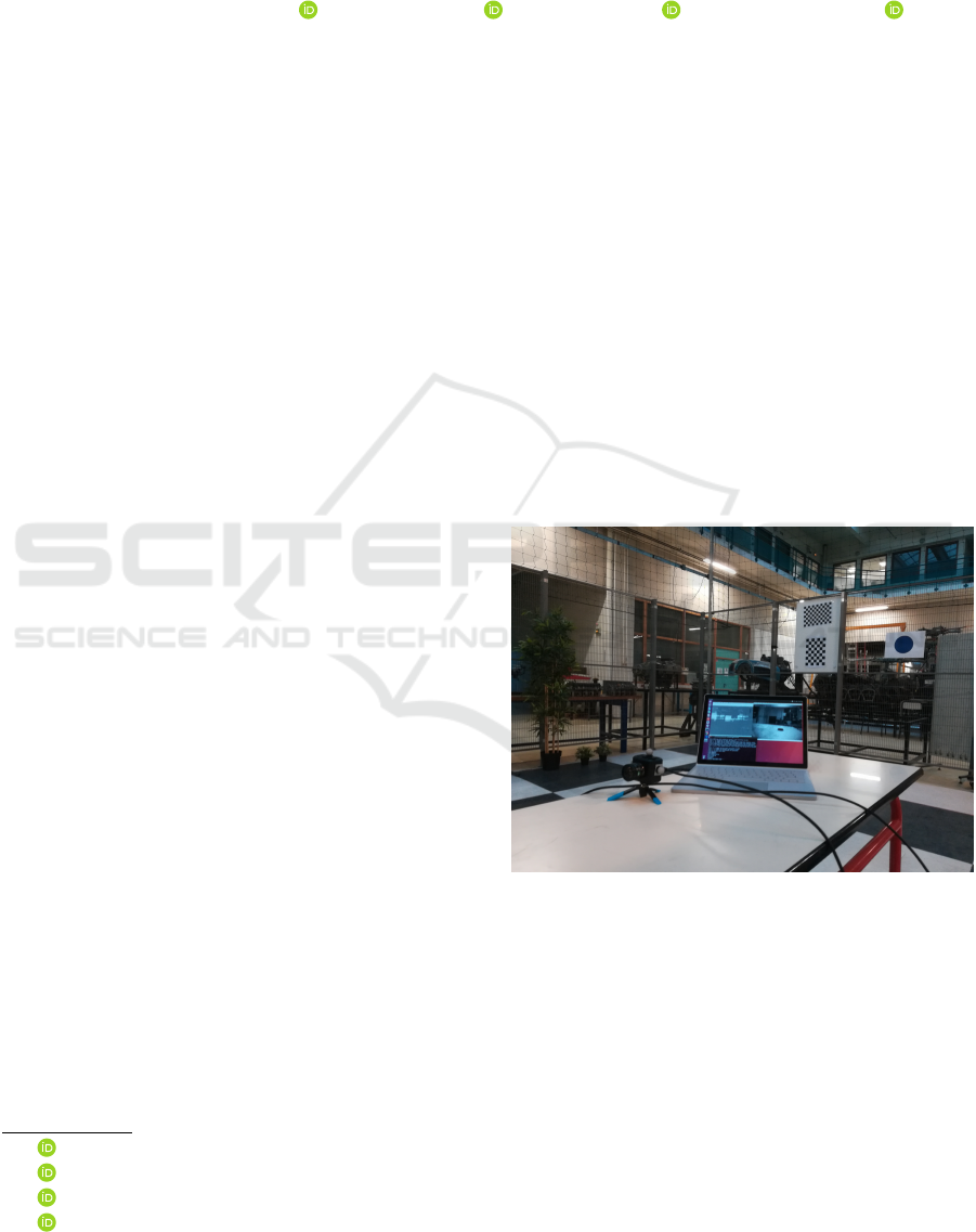
Figure 1: The environment setup of the system: event-based
camera, checkerboards, VICON system.
tem can provide a 6DOF pose ground truth with high
accuracy at frequencies above 100Hz while being
adapted to moving scenes with multiple moving ob-
jects. An optical flow ground truth can easily be de-
rived by measuring the relative objects-camera pose
to calculate the 2D objects projection on the camera
frame. We introduce a calibration method to align the
external VICON system with the DVS internal IMU
that can be applied easily for any sensors that share
roughly the same initial position. We also propose an
event-based data-set that can be used as ground truth
480
Khairallah, M., Bonardi, F., Roussel, D. and Bouchafa, S.
Data-set for Event-based Optical Flow Evaluation in Robotics Applications.
DOI: 10.5220/0010320304800489
In Proceedings of the 16th International Joint Conference on Computer Vision, Imaging and Computer Graphics Theory and Applications (VISIGRAPP 2021) - Volume 4: VISAPP, pages
480-489
ISBN: 978-989-758-488-6
Copyright
c
2021 by SCITEPRESS – Science and Technology Publications, Lda. All rights reserved

for optical flow algorithms comparison. Finally, we
evaluate existing event-based optical flow algorithms
that are adapted to robotics applications and previ-
ously introduced in (Delbr
¨
uck, 2008), (Benosman
et al., 2012), (Benosman et al., 2013), (Rueckauer and
Delbruck, 2016b) and (Mueggler et al., 2015). This
paper is organised as follows: in section 2, a brief
explanation of the selected optical flow algorithms is
presented. In section 3, an illustration of the recorded
data-set scenario is explained. In section 4 we present
the intrinsic and extrinsic calibration of the systems
and in section 5 a comparison between tested algo-
rithms estimated optical flows and the optical flow ob-
tained from VICON is carried out. Results and con-
clusion are given in the last sections.
2 EVENT-BASED OPTICAL
FLOW ALGORITHMS
Several optical flow algorithms have been developed
to adapt to the nature of event-based vision sensors
in robotics field. The algorithms presented in this
study can be grouped in three main categories: vari-
ants of Lucas-Kanade (Lucas and Kanade, 1981) op-
tical flow, Local Plane optical flow and Regularised
optical flow. We chose one algorithm from each cat-
egory according to efficiency and real-time robotics
applications adaptability criteria. Some modifications
are proposed to make these algorithms more adaptive
to different dynamic conditions.
2.1 Event-based Representation
The design of DVS cameras is particularly adapted
to the visual optical flow nature which is defined as
the perceived 2D motion of a 3D moving pattern.
The “silicon retina” used in DVS cameras mimics
the human eye derivative functionality (the system
responsible for motion detection) by sending a sig-
nal (event) whenever a change occurs at a specific
pixel. The created events can be characterized as a
tuple e = hx,y,t, pi where x and y are the position of
the event in pixel coordinates, t is the timestamp of
event’s creation and p is the polarity of the event such
that p ∈ {−1,+1}. The polarity of the event inter-
prets the increasing or decreasing change of illumina-
tion that occurs in the environment. An event is cre-
ated whenever a difference in illumination exceeds a
threshold according to the following equation:
∆L(x
i
,y
i
,t
i
) = L(x
i
,y
i
,t
i
) −L(x
i
,y
i
,t
i
−∆t) = p
i
δ
l
(1)
Figure 2: Left: events created due to motion of a beam dur-
ing 2 seconds without filtering. Right: events after filtering.
where L(x
i
,y
i
,t
i
) is the illumination log intensity of
the current time and L(x
i
,y
i
,t
i
−∆t) is the illumina-
tion log intensity of the event created at this pixel
previously at t
i
−∆t, δ
l
is the threshold that deter-
mines the creation of the event which is namely about
10 : 15%. The signed threshold δ
l
can be exceeded
due to change of luminosity in the environment with
no motion or due to motion under constant luminos-
ity or a combination of both cases. In robotics ap-
plications, we assume that environment luminosity
changes are negligible. Hence, under a brightness
constancy constraint, the creation of an event can be
approximated by the following equation using a Tay-
lor expansion of the intensity function:
∆L(x
i
,y
i
,t
i
) ≈
∂L
∂t
(x
i
,y
i
,t
i
)∆t = h∇
u
L(x
i
,y
i
,t
i
),
˙
u∆ti
(2)
where h.,.irefers to a dot product and ∇
u
L = (
∂L
∂x
,
∂L
∂y
).
The later equation shows that the creation of an event
embeds in itself the visual flow of the moving envi-
ronment. As a consequence, Event-Based cameras
provide a quasi-continuous flow of events which fa-
cilitates events correlation unlike standard cameras
which face brightness discretization issues. Accord-
ing to this, we give, in this study, a selection of Event-
Based optical flow algorithms that would be simple to
implement, running fast enough for real time applica-
tions and then we study their performance according
to different criteria. The selected approaches are pre-
sented in the following sub-sections.
2.2 Direction Selective Filter
(Delbr
¨
uck, 2008) propose to augment the information
that each event carries with a direction that is deter-
mined using a rough optical flow estimation. Veloc-
ity magnitude and direction are assigned to each event
through three steps: event filtering, direction selection
and magnitude estimation.
Data-set for Event-based Optical Flow Evaluation in Robotics Applications
481

2.2.1 Event Filtering
Due to the noisy nature and the sensitivity of DVS
cameras, it is essential to get rid of uncorrelated
events created by background activity or any other
source like transistor switch leakage (Lichtsteiner
et al., 2008). The author employs what is called an
activity filter to reject unwanted events that takes only
one parameter T , the “support time”, which is the
maximum time difference permitted between the cur-
rent event and events created previously in the same
neighbourhood. We use for that the active events
surface, which is the buffer that saves only the last
existing event at a specific pixel and its timestamp.
The support time T decides whether an event can be
passed as a true event or as noise. The process is
carried out in two steps. First, the event timestamp
is stored for the pixel 8-neighbourhood. Second, a
check between the timestamp stored in the event’s lo-
cation and the event’s timestamp is performed: if an
event occurred nearby the current event (within the
support time T), the new event is passed. It is dis-
carded otherwise.
Using a constant support time T is not the best
solution as events could be rejected or included ar-
bitrarily independently from the environment motion.
We propose a modified version of this filter to make
it more robust to noise and more adaptive to dynamic
environments. We thereby introduce an adaptive pa-
rameter T
f
that depends on the created events frequen-
cies since they are related to the dynamics of the en-
vironment. We use the concept of linear interpolation
to estimate T
f
so that it can be bounded by T
min
and
T
max
. Using the frequency directly would lead to be
stuck a narrow zone of T
f
. For this reason, we use
the log inverse function to exploit its saturation prop-
erty and stretch this zone according to the following
equations:
α =
k
log f
e
(3)
T
f
=
T
max
−T
min
α
max
−α
min
(α −α
min
) + T
min
(4)
where k is tuned to get a better logarithmic curve
and then the best value of T
f
for different frequen-
cies, T
min
and T
max
are the minimum and maximum
time period that the filter can provide. α
min
and α
max
are the values of α which correspond to the lowest
and highest values of events frequency f
e
. This fil-
ter was integrated to all the studied algorithms in this
paper to avoid computing incorrect optical flow from
noise events and losing time in unnecessary calcula-
tions (See Fig. 2).
2.2.2 Direction Selection
A moving edge will tend to create events that are very
close to each other in space and correlated in time.
The orientation filter treats the ON and OFF events
separately. The present event is given its correspond-
ing angle by checking the events that have the maxi-
mum correlation with the current event in the neigh-
borhood. Events correlation is defined as the differ-
ence in time between the current pixel and the pix-
els in the neighborhood, where events with maximum
correlation (and consequently minimum time differ-
ence) are necessarily created by the same edge. Ac-
cording to the location of these events the present
event is given a value among 4 possible orientations
separated by 45 degrees, one of four orientations is
assigned to an event but no positive or negative direc-
tion is assigned.
2.2.3 Magnitude Estimation
For the estimation of each event’s magnitude, the con-
cept of time of flight, introduced in (Rueckauer and
Delbruck, 2016a), is applied by computing the tem-
poral interval of the current event with the recent past
events along the direction of the edge. Since the di-
rection of the event is known at this step, it is used
to define the two directions perpendicular to the edge.
Time intervals of the pixels along that axis are com-
pared. Average of differences of each timestamp is
considered as the inverse of the speed on the events
(in pixel per second). A positive or negative direc-
tion is then assigned according to the time correlation
and considering that an edge will only create events
before the motion direction and not past it.
2.3 Adapted Lucas-Kanade Optical
Flow
The adaptation of Lucas-Kanade optical flow for
event-based vision sensors was first introduced by
(Benosman et al., 2012). The brightness constancy
constraint assumes that there is no change in bright-
ness w.r.t time i.e. d(I(x(t), y(t),t))/dt = 0 . This as-
sumption leads to the optical flow constraint equation
I
x
u + I
y
v = ∇I
T
·U = −I
t
where I
x
, I
y
and I
t
are the
partial derivatives of image intensity toward x, y and
t respectively, u and v are the components of the 2D
velocity vector in x and y directions respectively. As
the problem of optical flow defined in this scheme is
under-determined, an additional constraint was added
by Bruce D. Lucas and Takeo Kanade to solve it:
it consists of applying a neighbourhood consistency
condition. This condition uses the assumption that
VISAPP 2021 - 16th International Conference on Computer Vision Theory and Applications
482

neighbouring pixels will experience the same 2D ve-
locity. It employs a least-square optimisation scheme
to estimate the optical flow over a given neighbour-
hood.
2.3.1 Backward Finite Difference
The main challenge to estimate an event-based opti-
cal flow is to estimate image gradients I
x
, I
y
and I
t
.
The creation of an event requires a change of illumi-
nation (or gradient in case of illumination constancy)
that could be revealed by analyzing gradients values.
Thus, the gradient intensity is interpreted as the count
of events passed by a pixel during a fixed period of
time in the events space E(x,y,t). The events space
E(x,y,t) is the space of events that are created due
to environmental changes (motion or illumination).
(Benosman et al., 2012), propose a backward finite
difference scheme to obtain the equivalence of inten-
sity gradients using the following equation:
E
x
∼ H
e
(x
i
,y
i
,∆t) −H
e
(x
i
−1,y
i
,∆t) (5)
E
y
∼ H
e
(x
i
,y
i
,∆t) −H
e
(x
i
,y
i
−1,∆t) (6)
E
t
∼
H
e
(x
i
,y
i
,∆t) −H
e
(x
i
,y
i
,∆t)
t
i
−t
1
(7)
Where the subscripts x, y and t means the partial
derivatives in x, y and t directions respectively of
events mapping which is similar to image intensity.
The gradient is expressed to be similar to the notion
of sum of events that would fire at a specific pixel
compared to the sum of events fired at the neighbor-
ing pixel during an interval ∆t. H
e
is the histogram
of events which is the number of events created in a
specific pixel during a certain period of time .
2.3.2 Central Finite Difference
A bias in optical flow estimation is evident in the
backward scheme. (Rueckauer and Delbruck, 2016b)
introduce the central finite difference method which
would yield a symmetric gradient and eliminate the
backward bias of the basic Lucas-Kanade method.
For the 1
st
order method the events gradient became:
E
x
∼
1
2
(H
e
(x
i
+ 1,y
i
,∆t) −H
e
(x
i
−1,y
i
,∆t)) (8)
E
y
∼
1
2
(H
e
(x
i
,y
i
+ 1,∆t) −H
e
(x
i
,y
i
−1,∆t)) (9)
while no change has been introduced to the time gra-
dient estimation.
2.3.3 Savitzky-Golay Filter
Since the event-based Lucas-Kanade method is
mainly based on rate of event histograms (number of
events that occur at a certain pixel during a certain
interval of time) in a small neighborhood, the event
histogram does not gather a lot of events which would
lead to noise sensitivity. (Delbr
¨
uck, 2008) propose the
usage of Savitzky-Golay filter to estimate the image
gradient increasing as a consequence signal-to-noise
ratio. A low-order polynomial is introduced to fit ad-
jacent points using a least-square scheme, the fitted
two-dimensional polynomial function is described as:
SG(x,y) =
n
∑
p=0
n−p
∑
q=0
a
pq
x
p
y
q
(10)
where n represents the degree of the polynomial. The
order of the polynomial is chosen to be linear and
symmetric in both dimensions (namely first order),
SG(x,y) becomes a
00
+ a
01
y + a
10
x. The coefficients
a
00
, a
01
and a
10
are equivalent to the image gradients
E
t
, E
y
and E
x
. Coefficients a
pq
are obtained using a
least-square fit of data points: a = Cd d is a vector that
contains timestamp of events to be fitted. C is a ma-
trix calculated once for a certain size of neighborhood
and equal to C = (B
T
B)
−1
B
T
where B = x
p
y
q
is the
matrix containing the polynomial terms. Hence, the
least-square equation becomes a
pq
= (B
T
B)
−1
B
T
d.
After estimating the coefficients, the gradients can be
used to evaluate the optical flow while increasing the
SNR and also expecting a faster computation time.
2.4 Local Plane Fit Optical Flow
By exploiting the almost-continuous nature of the cre-
ated events from event-based cameras (created events
would look like an extruded shape extended in time
using edges, See Fig. 3), it helps a lot to estimate im-
age gradients accurately. The local plane fit scheme
aims to estimate a vector n
p
perpendicular to the local
plane around each event. The directional components
of this vector enclose the spatial and temporal infor-
mation of the moving edge that triggered this event.
(Benosman et al., 2013) formulated this scheme by
using the concept of events mapping.
∑
e
: N
2
7→ R (11)
(x,y) 7→
∑
e
(x,y) = t (12)
Where events pixel coordinates (x,y) are mapped
along the time axis t.
2.4.1 Iterated Fit
Since time is a monotonically increasing function of
space we can assert that the partial derivatives of
∑
e
are non zero increasing functions, then the usage of
Data-set for Event-based Optical Flow Evaluation in Robotics Applications
483

Figure 3: Events Plane-like shapes due to a beam motion
(planes correspond to different edges of the beam).
the inverse function theorem around each event is pos-
sible as
∑
ex
(x,y
0
) =
d
∑
e|y
0
dx
=
1
v
x
(x,y
0
)
(13)
∑
ey
(x
0
,y) =
d
∑
e|x
0
dy
=
1
v
y
(x
0
,y)
(14)
where ∇
∑
e
= (
1
v
x
,
1
v
y
) is the change gradient vector of
time w.r.t space. At each event arrival, a plane is fitted
to get the optical flow values using the events packed
in a spatio-temporal local neighborhood of L ×L ×
2∆t. The event under test is used as the center of this
neighborhood, accordingly, a plane equation should
be satisfied within a σ
1
threshold. Each event fits a
plane as in:
ax + by + ct + d = 0 (15)
where (a b c d)
T
are the plane parameters. After fit-
ting a plane for the present event with its neighbor-
hood, a check is carried out to make sure that all
events belong to the same surface of the plane within
a threshold σ
2
. In case an event does not belong to
the surface, it is rejected and the same process is re-
peated until a plane fits within the specified threshold
where the optical flow components are v
x
= −c/a and
v
y
= −c/b.
2.4.2 Robust Single Fit
We apply the iterations to make sure that all the events
belong to the estimated surface impose a strict con-
ditions that would lead to performance deterioration.
(Rueckauer and Delbruck, 2016b) propose to use only
a single fit while changing the optical flow equations
to be
v
x
v
y
=
1
|g|
2
g =
−c
a
2
+ b
2
a
b
(16)
where g (
−a
c
−b
c
)
T
is the gradient to avoid infinity val-
ues of optical flow .
2.4.3 Savitzky-Golay Plane Fit
To add a smoothing effect on a noisy events plane sur-
face, a Savitizky-Golay two-dimensional filter is ap-
plied to obtain the plane parameters the same way it
is used in Lucas-Kanade (see 2.3.3) while some mod-
ifications to map a plane are applied. a
pq
is calculated
from the least-square scheme. The plane equation is
considered with c = −1. The polynomial equation
SG(x,y) = a
00
+ a
01
y + a
10
x is now mapped to the
plane equation ax + by + ct + d = 0.
2.4.4 Regularised Plane Fit
To speed up the computation of the local plane fit
algorithm and get higher accuracy, (Mueggler et al.,
2015) use RANSAC instead of the optimization algo-
rithm while reducing the neighborhood to be L ×L ×
∆t, taking into account only events created prior to
the present event. They use a local plane fit and a reg-
ularization step to refine events’ lifetime estimation,
where the lifetime is the time of existence of an event
after its creation and defined as:
√
a
2
+ b
2
/c. The out-
put of the plane fitting algorithm is then used as input
of the regularization scheme to smooth the estimated
plane parameter by enforcing optimization in the tem-
poral direction. The assumption of constant velocity
is used to predict the lifetime of the event in the flow
direction
ˆ
t
e
. The error term to be used is defined as a
measure of confidence of local plane fit estimation:
∆t
err
= |t
e
−
ˆ
t
e
| (17)
so the regularized plane vector is
n
R
= arg min(||An −b||
2
+ λ(∆t
err
)||n −
ˆ
n
i
||
2
) (18)
where n is the estimated plane parameters vector
(
a
d
b
d
c
d
) and
ˆ
n
T
i
is the predicted one obtained from
neighbourhood events. The term ||An − b|| is the
least-square error of the local plane fit where b is a
vector of ones (equation 15 normalized w.r.t d). The
regularization term λ(∆t
err
) is an empirical function
of ∆t
err
mainly used to refine events’ lifetime. The
usage of plane normal drives the regularization to
smooth the optical flow estimation as well while fo-
cusing the optimization on the time component. This
guarantees a smoother but not necessarily an optimal
performance for optical flow estimation.
3 DATA-SET SCENARIOS
In order to have a quantitative evaluation of the pre-
sented algorithms, an optical flow ground truth should
be provided. The paradigm shift influenced by DVS
cameras requires new approaches to create optical
flow ground-truth while assuring very fine accuracy
which is rarely found in the state of the art. For
these reasons, we exploit VICON system endowed
VISAPP 2021 - 16th International Conference on Computer Vision Theory and Applications
484
with high precision and accuracy and employed a new
methodology to create the ground truth. The VICON
system tracks the PROPHESEE event-based camera
that also provides IMU readings to create the needed
data-sets. In order to test the reliability of the devel-
oped algorithms, datasets featuring in-plane rotation,
in-plane translation both at various speeds and also a
free-hand motion scenario have been recorded. In all
these scenarios, the camera is moving in front of a
tracked checkerboard. Checkerboard rigid transform
relative to the camera is obtained with the VICON
tracking system allowing us to project the checker-
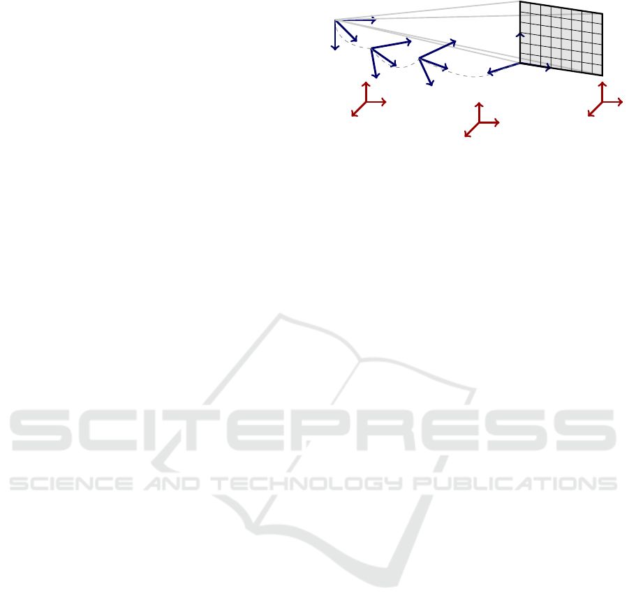
board grid in a camera frame. Reference frames of our
experimental setup are explained in Fig. 4. The goal
of the various scenarios is to better understand the ca-
pabilities and shortcomings of each implemented al-
gorithm. Fig. 1 shows the real environmental setup of
our dataset.
4 SENSORS CALIBRATION
The VICON system is calibrated easily using the pro-
vided software and it returns the states of the point of
origin of the board along with the camera pose. How-
ever, our goal is to obtain apparent motion ground
truth suitable to optical flow evaluation rather than
extrinsic parameters of the camera as used in SLAM
or visual-odometry. And since tested algorithms will
only provide apparent motion, we propose to make
use of the camera’s embedded IMU as a middle trans-
formation to estimate between the VICON and the
camera frames so that the transformations for the
markers on the board and on the camera are (see Fig.
5):
T
c
vic
= T
c
IMU
×T
IMU
vic
(19)
T
c
B
= T
c
IMU
×T
IMU
vic
×T
vic
B
(20)
4.1 Intrinsic Calibration
Camera and IMU need to be intrinsically calibrated
before implementing the extrinsic calibration.
4.1.1 IMU Intrinsic Calibration
To understand the IMU intrinsic calibration, we need
to point out that the IMU parameters to be estimated
are divided into two categories, deterministic and ran-
dom. Deterministic parameters are scale factor, mis-
alignment error and bias offsets. Random errors are
the bias residuals and white noise added to the signal,
Y
c
X
c
Z
c
O
c
Z
IMU
Y
IMU
X
IMU
O
IMU
X
gt
Z
gt
Y
gt
O
gt
Y
B
X
B
Z
B
O
B
T
C
IMU
T
IMU
vic
T
vic
B
X
vic
Y
vic
Z
vic
O
vic
X
W
Y
W
Z
W
O
W
X
V
Y
V
Z
V
O
V
Figure 4: Different reference frames (fixed and moving).
the IMU can be modeled as follows:
ω
IMU
= [I + M
g
]ω + b
g
+ δb
g
+ ε
g
(21)
a
IMU
= [I + M
a
]a + b
a
+ δb
a
+ ε
a
(22)
where ω
IMU
and a
IMU
are 3D vectors, rotational ve-
locity and acceleration obtained by the IMU. M
g
and
M
a
are the matrices that contains misalignment errors
of the gyroscope and accelerometer respectively. b
g
and b
a
are the offset bias of the gyroscope and ac-
celerometer. δb
g
and δb
a
are the bias residual of the
gyroscope and accelerometer that changes with very
low frequency. ε
g
and ε
a
are white noise of the gyro-
scope and accelerometer respectively. Using the six-
position calibration (El-Diasty and Pagiatakis, 2010),
we obtain the deterministic parameters of the IMU ex-
cept for the matrix M
g
because of the inability to have
accurate known excitation source for the gyroscope,
which still can be suppressed in a scheme of fusion.
We use Allan variance modeling (El-Sheimy et al.,
2007) in order to estimate the parameters that controls
the modeling of random IMU parameters.
4.1.2 Camera Intrinsic Calibration
The process of calibrating an event-Based camera is
similar to the process for standard cameras, except in
the image creation phase. In order to overcome the
nature of event-based cameras, we use flashing pat-
terns to adjust the sharpness and lens focus. We gen-
erate a flashing checkerboard on a screen and use the
resulting images as an input for the embedded MAT-
LAB camera calibrator toolbox to estimate the intrin-
sic parameters of the camera.
4.2 Extrinsic Calibration
The VICON system and camera need to be calibrated
both spatially and temporally. The extrinsic calibra-
tion process is divided into temporal synchronization
and spatial alignment to make sure the outputs from
different systems are adjusted perfectly.
Data-set for Event-based Optical Flow Evaluation in Robotics Applications
485
Algorithm 1: IMU-VICON Calibration.
Data: {Θ
IMU
}
N−1
i=0
, {Θ
vic
}
N−1
i=0
Result: q , ∆t
1 Initialize: check = true , itr = 1 , ε = small value
2 while check = true do
3 µ
IMU
=
1
N
N−1
∑
i=0
Θ
IMU
i
, µ
vic
=
1
N
N−1
∑
i=0
Θ
vic
i
4 Θ
IMU
= Θ
IMU
−µ
IMU
, Θ
vic
= Θ
vic
−µ
vic
5 Calculate: S
mn
=
N−1
∑
i=0
Θ
IMU
m
Θ
vic
n
9 values
6 Construct: N
4×4
matrix see (Sola, 2017)
7 Solve: {λ,V } = eig(N)
8 q
itr
= V
λ
1
q is the vector corresponds to maximum λ
9 project: Θ
MU
= R
q
Θ
IMU
10 Solve: ∆t
itr
= xcorr(Θ
IMU
,Θ
vic
)
11 Shift: Θ
IMU
= Θ
IMU
(∆t : end)
12 itr + +
13 if
1
N
N−1
∑
0
|Θ
IMU
i
−Θ
vic
i
| < ε then
14 check = false
15 end
16 end
17 q =
itr
∏
n=1
q
n
18 ∆t =
itr
∑
n=1
∆t
n
4.2.1 VICON-IMU Extrinsic Calibration
The correspondence problem of two different frames
of reference that observe the same states are widely
known as Wahba’s problem (Wahba, 1965), where the
author defined it, for given two 3D sets of measure-
ments {X
i
}
N−1
i=0
and {Y
i
}
N−1
i=0
, as the least square mini-
mization of
argmin
{s,R,t}
N−1
∑
i=0
|Y
i
−s(RX
i
+ t)|
2
(23)
where s, R ant t are scale, rotation and translation be-
tween the two frames respectively. The main two as-
sumptions in order to be able to solve this minimiza-
tion problem are that noise is suppressed in both mea-
surements and that they are temporally synchronized.
Since the IMU measurements suffer from high noise
due to integration effect, we choose to use the angles
to be injected in the minimization problem. We use
an error state Kalman filter (Sola, 2017) to obtain the
accurate measurements. To solve the alignment prob-
lem, we adopt an iterative scheme since each of the
spatial and temporal alignments needs one another as
a prerequisite to be fulfilled. We solve for an initial
transformation between the two frames using Horn’s
reformulation of Wahba’s problem (Horn, 1986) (see
algorithm 1).
argmin
q
N−1
∑
i=0
(q ×Θ
IMU
×q
∗
)Θ
vic
(24)
where Θ
IMU
and Θ
vic
are the angles measured in IMU
and VICON frames and q is a unit quaternion that
represents a rigid body transformation. We project
the IMU readings in the VICON frame to apply cross
correlation between the two signals to find ∆t that
would temporally align them. We repeat until the dif-
ference between the estimated calibration parameters
reaches convergence. It is noted that after two itera-
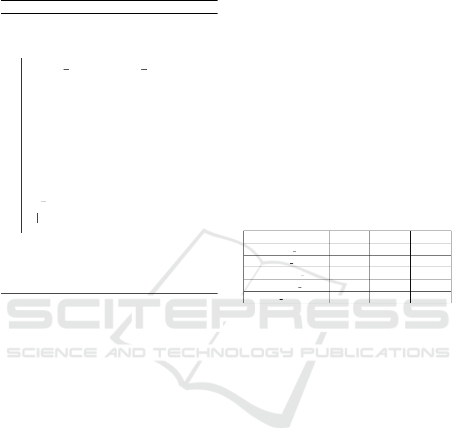
tions, convergence is fulfilled. Fig. 5 shows IMU and
VICON measured angles before and after calibration.
To make sure that every sequence is correctly corre-
lated, we calculate the mean absolute difference be-
tween the VICON angles and IMU angles after being
transformed in VICON frame, results are shown in
Table 1.
Table 1: VICON / IMU angles comparison.
sequence φ[
◦
] θ[
◦
] ψ[
◦
]
rotate low 0.7893 0.5988 1.5579
rotate high 1.2885 0.9427 0.4945
translate low 1.2347 1.5135 0.4813
translate high 1.4031 1.6943 0.4838
free motion 0.3923 0.5544 0.3923
4.2.2 Camera-IMU Calibration
After getting the spatio-temporal calibration between
the VICON and IMU we need to do the same between
the IMU and the Camera. We used Kalibr toolbox
(Furgale et al., 2014) to get the spatial transforma-
tion between the camera and the IMU. Since Kalibr
provides a temporal difference only for the provided
data-set used for calibration (which was totally differ-
ent from the data-set used for our comparison), we use
the concept of cross correlation between the IMU ab-
solute rotational velocity and the events frequency in
order to find the best time shift. The choice of events
frequency to be correlated with absolute rotational ve-
locity is similar to the temporal synchronization used
in (Censi and Scaramuzza, 2014) since with a higher
velocity more events would be triggered per second,
so the best synchronization will correspond to the best
matching these two signals together.
5 GROUND TRUTH CREATION
AND COMPARISON
Next step after calibration is to recreate accurate
events positions of the checker board to be projected
VISAPP 2021 - 16th International Conference on Computer Vision Theory and Applications
486
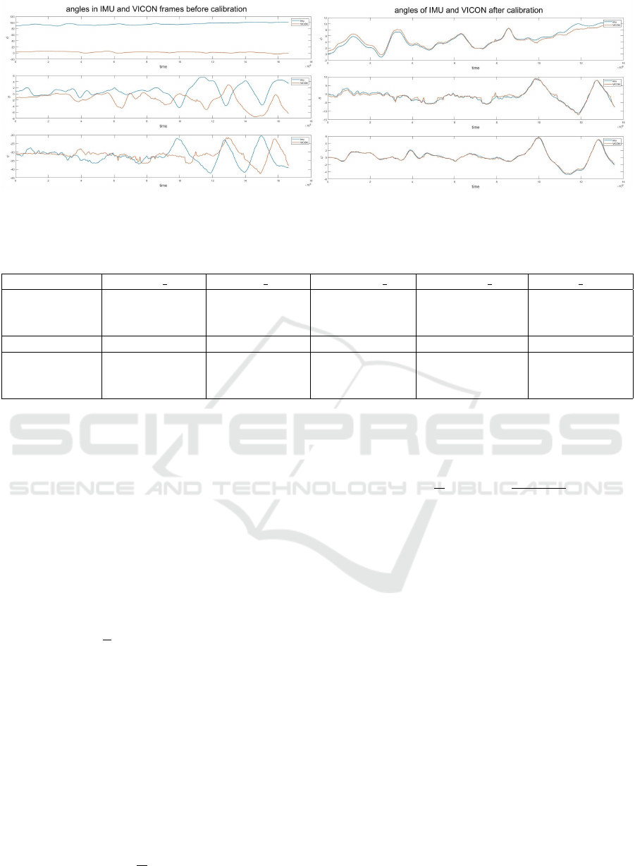
Figure 5: Left: an example of angles (namely the roll angle) in VICON and IMU frames without alignment. Right: the angles
after being transformed in the IMU frame is shown to be perfectly aligned.
Table 2: Average angular error of evaluated algorithms in degrees (DS stands for Direction Selective filter, LK for Lucas-
Kanade, LP for Local Plane fit and SG for Savitsky-Golay).
Algorithm rotate low rotate high translate low translate high move free
LK Backward 35.158 ±27.547 41.585±15.715 32.314 ±12.642 35.526 ±12.642 22.975 ±23.839
LK Central 23.587 ±19.481 21.135±17.161 19.135 ±10.362 20.264 ±9.321 18.625 ±20.881
LK SG 16.754 ±9.571 15.487 ±10.131 14.361 ±3.752 13.595 ±8.839 10.576 ±11.935
DS 78.391 ±20.507 71.775±21.781 53.651 ±17.432 57.205 ±19.381 72.890 ±68.497
LP Single Fit 12.835 ±5.718 14.304 ±5.203 6.914 ±3.567 6.937 ±4.893 9.350 ±7.761
LP SG 8.905 ±3.107 7.751 ±4.978 5.744 ±2.742 5.065 ±1.347 8.678 ±7.271
LP Regularized 5.871 ±4.178 6.170 ±4.108 5.863 ±3.108 4.709 ±2.938 18.707 ±15.463
in the camera frame using equation 20. We create 3D
points which reside on the edges of the 9×7 checker-
board at time t
0
and then transform these points at
each time step in the camera frame. The intrinsic
calibration is used to project the transformed checker-
board in the pixels frame while undistorting the scene.
To create the optical flow ground truth values, we fol-
low (Heeger and Jepson, 1992) proposition, exploit-
ing the fact that the checkerboard is a rigid plane. If
we have V and W as translation and rotation speeds
of the 3D scene then the optical flow will be approxi-
mated by the 2D projection of the 3D motion accord-
ing to the equation:
U(x,y) =
1
Z
A(x,y)V + B(x, y)W (25)
where,
A(x,y) =
−f 0 x
0 −f y
(26)
B(x,y) =
(xy)/ f −( f + x
2
/ f ) y
( f + x
2
/ f ) −(xy)/ f −x
(27)
With the created ground truth, we adopt the met-
rics in (Baker et al., 2011) for quantitative compari-
son. First metric is the average endpoint error (AEPE)
which is defined as the average value of the vector dis-
tance between the estimated motion u and the ground-
truth
ˆ
u:
AEPE =
1
N
N
∑
i=1
||u
i
−
ˆ
u
i
|| (28)
The second metric is the average angular error (AAE)
which is defined as the average angle between the es-
timated motion u and the ground truth
ˆ
u:
AAE =
1
N
N
∑
i=1
cos
−1
ˆ
u
T
i
u
i
||
ˆ
u
i
||||u
i
||
(29)
To make sure that the created data-set are reliable and
that any calibration error is omitted, we randomly se-
lect two consequent VICON frames f
1
and f
2
and use
the optical flow ground truth to project events trig-
gered between those two frames to the frame f
2
(see
Fig. 7). We use the mean of absolute difference be-
tween the projected events and the created frame as an
error metric. Errors after events projection show ac-
ceptable results where the projected events are aligned
with the boundaries of the synthetic board and the
mean of absolute difference did not exceed the bound
of 2 pixel. (see Fig.6)
6 RESULTS
In order to show the comparison between the different
algorithms without being biased with high value er-
rors, we use the mean and variance of optical flow val-
ues to remove extreme outliers. We apply the compar-
ison w.r.t accuracy and computational power needed.
Results are demonstrated in Tables 2 and 3 . Since
Data-set for Event-based Optical Flow Evaluation in Robotics Applications
487
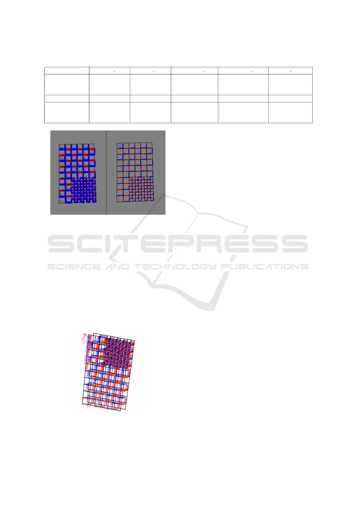
Table 3: Relative average end point error of the evaluated algorithms.
Algorithm rotate low rotate high translate low translate high move free
LK Backward 1.324 ±0.607 1.215 ±0.749 0.934 ±0.691 0.883 ±0.482 1.196 ±0.405
LK Central 1.057 ±0.254 0.951 ±0.512 0.894 ±0.533 0.811 ±0.328 1.163 ±0.677
LK SG 0.921 ±0.421 0.812 ±0.458 0.664 ±0.582 0.521 ±0.387 0.994 ±0.369
DS 1.721 ±0.227 1.851 ±0.554 1.322 ±0.363 1.391 ±0.452 1.679 ±1.2161
LP Single Fit 1.125 ±0.248 1.054 ±0.187 0.891 ±0.155 0.803 ±0.183 1.286 ±0.320
LP SG 0.681 ±0.384 0.621 ±0.321 0.347 ±0.124 0.382 ±0.168 0.691 ±0.456
LP Regularized 0.755 ±0.327 0.604 ±0.247 0.404 ±0.203 0.410 ±0.137 0.999 ±0.010
Figure 6: (Left) the events and the synthetic created
checkerboard before projecting the events using the optical
flow ground truth, (Right) the projected on and off events
in the camera frame are sufficiently aligned with the cre-
ated checkerboard where the mean of absolute difference
did not exceed the bound of 2 pixel.
algorithms have been tested using MATLAB, com-
putation time in itself is not a significant metric but
relative differences between algorithms indicate the
computational power needed.
6.1 Average Angular Error
The obtained results show that the Direction Selec-
tion filter has -as expected- the lowest angular er-
ror accuracy in all the tested sequences since it pro-
Figure 7: In black: two consequent frames created by the
projection of the VICON system. Positive triggered events
are shown in red and negative events in blue.
vides only a notion of the motion in 8 discrete direc-
tions. In the three categories of algorithms, we can
conclude that the Local Plane algorithms outperform
the other algorithms. The addition of optimal regu-
larization significantly refine the estimation of opti-
cal flow’s direction but did not provide the best es-
timation for all sequences because the regularization
term optimizes only the temporal component of the
plane’s normal and not the spatial components. The
usage of Savitsky-Golay filter enhances the accuracy
of angular error which did not vary much compared
to the Regularized plane fit. The performance of the
algorithms under test was shown to be always better
for scenarios featuring translations while noting that
the Regularized plane fit always provide better per-
formance than Savitsky-Golay Local Plane fit because
the smoothness effect may not be prominent if the op-
tical flow varies much in neighbourhoods which is the
case while rotating.
6.2 Average End Point Error
Using the Direction Selective filter feature the least
accuracy due to the lack of events used to estimate the
optical flow. Savitsky-Golay Local Plane fit is seen to
always provide better endpoint error (except for high
rotation sequences with minor difference). Regulariz-
ing the local plane optical flow helps to enhance the
end point error but could not exceed the accuracy of
Savitsky-Golay filter for the reason mentioned in the
previous section that the regularization enforces only
temporal accuracy.
6.3 Computation Time
Although the Direction Selection filter did not pro-
vide the best accuracy, it was the fastest algorithm to
be performed with significantly shorter computation
time, which means that it can be used as indication
or as a preliminary step to add direction information
for each event. On the other hand, using Regulariza-
tion -while not being the best w.r.t performance in all
the cases- add a significant rise in computation time.
Because of this aspect, we question the relevance of
VISAPP 2021 - 16th International Conference on Computer Vision Theory and Applications
488

Table 4: Computation times needed for calculations per
event.
algorithm computational time [µs]
DS 77.465 ±32.540
LK Backward 312.974 ±170.568
LK Central 384.489 ±184.946
LK Savitzky-Golay 264.913 ±94.412
LP Single Fit 173.89 ±120.973
LP Savitsky-Golay 129.749 ±112.549
LP regularized 536.486 ±173.914
integrating this algorithm in a more complex scheme.
The Lucas-Kanade algorithm provides relatively good
error accuracy but is not the best in terms of compu-
tational cost. Presenting Savitsky-Golay filter for any
algorithm (Lucas-Kanade or Local Plane fit) always
refines the accuracy while significantly reducing com-
putation time.
7 CONCLUSION
In this paper, we present a methodology to compare
state-of-the-art event-based optical flow algorithms
and show their performance in the context of robotic
applications. The suggested evaluation led us to pro-
pose an event-based optical flow ground-truth data-
set using a VICON system. Our study reveals that
all the evaluated algorithms need a lot of tuning w.r.t
the time interval to calculate optical flow while also
tuning many thresholds to get the best optical flow
values. Our future work will then focus on proposing
adaptive solutions to make these algorithms perform
better for various scenes in robotic applications while
improving their global performance.
REFERENCES
Baker, S., Scharstein, D., Lewis, J., Roth, S., Black, M. J.,
and Szeliski, R. (2011). A database and evaluation
methodology for optical flow. International journal
of computer vision, 92(1):1–31.
Barranco, F., Fermuller, C., Aloimonos, Y., and Delbruck,
T. (2016). A dataset for visual navigation with neuro-
morphic methods. Frontiers in neuroscience, 10:49.
Benosman, R., Clercq, C., Lagorce, X., Ieng, S.-H., and
Bartolozzi, C. (2013). Event-based visual flow. IEEE
transactions on neural networks and learning systems,
25(2):407–417.
Benosman, R., Ieng, S.-H., Clercq, C., Bartolozzi, C.,
and Srinivasan, M. (2012). Asynchronous frameless
event-based optical flow. Neural Networks, 27:32–37.
Censi, A. and Scaramuzza, D. (2014). Low-latency event-
based visual odometry. In 2014 IEEE International
Conference on Robotics and Automation (ICRA),
pages 703–710. IEEE.
Delbr
¨
uck, T. (2008). Frame-free dynamic digital vision. In
Proceedings of International Symposium on Secure-
Life Electronics, Advanced Electronics for Quality
Life and Society, Univ. of Tokyo, Mar. 6-7, 2008, pages
21–26. nternational Symposium on Secure-Life Elec-
tronics, Advanced Electronics for . . . .
El-Diasty, M. and Pagiatakis, S. (2010). Calibration and
stochastic m odelling of i nertial na vigation s ensor er-
rors. Positioning (POS) Journal Information, page 80.
El-Sheimy, N., Hou, H., and Niu, X. (2007). Analysis
and modeling of inertial sensors using allan variance.
IEEE Transactions on instrumentation and measure-
ment, 57(1):140–149.
Furgale, P., Maye, J., Rehder, J., and Schneider, T. (2014).
Kalibr: A unified camera/imu calibration toolbox.
Heeger, D. J. and Jepson, A. D. (1992). Subspace methods
for recovering rigid motion i: Algorithm and imple-
mentation. International Journal of Computer Vision,
7(2):95–117.
Horn, B. K. P. (1986). Closed-form solution of absolute
orientation using uni t quaternions.
Lichtsteiner, P., Posch, C., and Delbruck, T. (2008). A
128×128 120 db 15µ s latency asynchronous tempo-
ral contrast vision sensor. IEEE journal of solid-state
circuits, 43(2):566–576.
Lucas, B. D. and Kanade, T. (1981). An iterative image
registration technique with an application to stereo vi-
sion. In IJCAI.
Menze, M., Heipke, C., and Geiger, A. (2015). Joint 3d esti-
mation of vehicles and scene flow. In ISPRS Workshop
on Image Sequence Analysis (ISA).
Mueggler, E., Forster, C., Baumli, N., Gallego, G., and
Scaramuzza, D. (2015). Lifetime estimation of events
from dynamic vision sensors. In 2015 IEEE in-
ternational conference on Robotics and Automation
(ICRA), pages 4874–4881. IEEE.
Rueckauer, B. and Delbruck, T. (2016a). Evaluation of
event-based algorithms for optical flow with ground-
truth from inertial measurement sensor. Frontiers in
neuroscience, 10:176.
Rueckauer, B. and Delbruck, T. (2016b). Evaluation of
event-based algorithms for optical flow with ground-
truth from inertial measurement sensor. Frontiers in
neuroscience, 10:176.
Sola, J. (2017). Quaternion kinematics for the error-state
kalman filter.
Wahba, G. (1965). A least squares estimate of satellite atti-
tude. SIAM review, 7(3):409–409.
Data-set for Event-based Optical Flow Evaluation in Robotics Applications
489
